QuestDB 10.0: QWP, one binary streaming protocol for writes and Arrow reads
QuestDB 10.0 ships QWP, a binary columnar protocol that both writes data in and streams Arrow back out, from a single client. It also brings live views in beta, notebooks driven by coding agents, and the storage work that QuestDB Enterprise 4.0 builds cold storage on.



Fast ingestion is what QuestDB is known for. Getting the data back out at the same speed was the harder problem, and for years the answer was the PostgreSQL wire protocol, which was never designed for it.
10.0 closes that gap, and speeds up the write side on the way past. QWP, the QuestDB Wire Protocol, is a binary columnar protocol over WebSocket that handles both writes and reads from a single client: around 3.6x faster than the InfluxDB Line Protocol ("ILP") for ingestion over a network, and query results streaming into Apache Arrow at 220 million rows a second.
There is a good deal more in the release. Live views arrive in beta, the Web
Console gains notebooks that a coding agent can drive, ALTER COLUMN TYPE works
on Parquet partitions, and the storage engine gains the foundations that QuestDB
Enterprise 4.0 builds cold storage on.
It is a long post, so here is what is in it:
- One protocol, both directions: QWP on the write side and the read side, the benchmarks, and what ships in which client
- Live views, in beta: window functions maintained incrementally in memory as rows arrive
- Parquet as a first-class citizen: Parquet tables, schema evolution on them, and files the rest of the ecosystem can read
- Cold storage, and the lakehouse it opens up: partitions tiered to object storage in QuestDB Enterprise 4.0, still queryable, and registrable in Iceberg or DuckLake without a copy
- Notebooks, and coding agents that can drive them: Web Console 2.0 and the QuestDB MCP
- The covering index gets its parallel decode: the 9.4.0 caveat, closed
- New SQL features:
SHOW CREATE DATABASE, scalar sub-queries in comparisons, and a few new functions - Operations: per-query memory limits, cancellation that works,
REBASE WAL - Performance and breaking changes
- Bug fixes, and the fuzzer behind them
- Getting 10.0
One protocol, both directions
Getting data in meant ILP, and getting it back out meant the PostgreSQL wire protocol: two libraries, two wire formats, and one of them serialising every row to text on the server for the client to parse back into typed values. Fine for a dashboard query returning forty rows, a bottleneck when a quant pulls a year of ticks into pandas.
QWP is a better alternative to both halves. It is binary and columnar, sending whole column blocks in close to the shape they live on disk, with symbols sent once and referenced by an id and timestamps delta encoded. Query results come back as Apache Arrow record batches, which makes handing them to polars or pandas zero copy: the bytes off the socket are already in the layout those libraries use, with no row-by-row deserialising in between.
There is more to it than speed. The QWP clients also handle buffering and node failover themselves, with no queue or proxy in front of QuestDB, which is further down.
That does not make the older paths go away. ILP and the PostgreSQL wire protocol are both still here, still supported, and nothing you run today stops working when you upgrade. ILP in particular is simple, well optimised, and spoken by a wide range of tools and older QuestDB versions, and we have no plans to retire it. If you have a Telegraf agent or a Grafana datasource pointed at QuestDB, it keeps working exactly as before.
Switching is a connect-string change rather than a rewrite, because it is the
same client library either way. Sender.fromConfig() takes http:: or tcp::
for ILP and ws:: or wss:: for QWP, and the builder API around it is
unchanged:
// ILP over HTTP, as beforeSender sender = Sender.fromConfig("http::addr=localhost:9000;");// QWP over WebSocketSender sender = Sender.fromConfig("ws::addr=localhost:9000;");
Which means you can move one service at a time, and move it back if you do not like what you see.
Ingestion
We benchmarked QWP against ILP with TSBS, the standard Time Series Benchmark Suite, feeding both protocols wire data prepared ahead of time so neither gets a serialisation head start.
↑ Higher is better
TSBS cpu-only at 1,000,000 hosts, wire data prepared ahead of time for both protocols
over the network
on a single machine
distinct series
The gain is mostly the format. A TSBS row is around 347 bytes as line protocol text and around 97 bytes as QWP. Both protocols fill the same 14.7 Gbit/s link, so the one with the smaller rows gets about 3.6x more of them through. The full ingestion benchmark has the cardinality sweep, the methodology, and why running the loader on the same box as the server makes the two protocols look level.
Egress
On the read side we measured how fast a Python client can drain a 500 million row table into Arrow, against ClickHouse and TimescaleDB on the same hardware, each engine at the fastest configuration we could find for it.
↑ Higher is better
Each engine at its own fastest measured configuration, 500M rows, 8 parallel readers
vs ClickHouse native
vs ClickHouse Arrow
to the first Arrow batch
That is 500 million rows drained in 2.3 seconds, with the first Arrow batch
landing after 32 milliseconds. QuestDB also moves the fewest bytes per row, 18.8
against 21.4, 27.0 and 64.3, because SYMBOL columns cross the wire as Arrow
dictionaries rather than repeating the same strings half a billion times.
ClickHouse appears twice because its fastest buffering path and its fastest streaming path are not the same one. The 141.9M configuration materialises about 18 GB in the client and returns nothing for 15.3 seconds, then everything at once. Against its fastest configuration of any kind QuestDB is 1.55x ahead, and against its fastest streaming one, 2.35x.
Each benchmark gets its own post, with the full methodology, the tables behind these charts, the caveats, and the harnesses to reproduce them. The ingestion one is out now, and the egress one follows shortly. Several of our own early conclusions in both turned out to be artifacts of the test rig rather than facts about any database, and the posts say so.
One client for both
In practice you stop needing an ingestion library and a separate PostgreSQL driver. One dependency and one connect string, with a single handle that writes and reads:
import questdbfrom questdb import TimestampNanoswith questdb.connect("ws::addr=localhost:9000;") as db:with db.sender() as sender:sender.row("trades",symbols={"symbol": "ETH-USDT"},columns={"price": 2615.54, "amount": 0.00044},at=TimestampNanos.now(),)sender.flush()with db.query("SELECT timestamp, symbol, price FROM trades WHERE symbol = $1",["ETH-USDT"],) as result:frame = result.to_polars()
There are to_pandas() and to_arrow() equivalents, along with streaming
variants for results too large to hold in memory, and db.dataframe() going the
other way for data that is already in columns.
Client availability
| Client | QWP status |
|---|---|
| Java, C/C++, Rust, Python | Full support |
| Go, .NET | Beta. Most QWP features, not full compatibility yet |
| Node.js | Coming in a later release |
A production Go and .NET release follows shortly after 10.0. Node.js and any client not listed as full support keep their existing ILP and PGWire paths in the meantime, so a language without QWP yet is no worse off than it is today.
Store-and-forward and failover
What happens to your writes when QuestDB is not there to take them? Normally that becomes your problem, and you end up putting a queue in front of the database or writing retry logic and hoping you got it right.
Store-and-forward means the client does it for you. It holds on to any rows the
server has not confirmed, reconnects when the connection drops, and sends them
again. Your code keeps calling row() and never blocks on the network. The
buffer can be kept on disk instead of in memory, so the rows also survive the
producer itself crashing.
Failover is the same idea applied to nodes. Put more than one host in the connect string and the client moves to another when one goes away, without your code noticing. On the read side that is useful in plain OSS, where a hot/hot pair keeps serving queries through a node loss. Consistent failover for writes is where QuestDB Enterprise replication comes in, and 10.0 adds a hot in-place primary/replica role switch on that side, so promoting a replica no longer needs a restart.
See store-and-forward and client failover for the full picture, and the wire protocol specs if you are implementing a client.
Live views, in beta
Live views incrementally maintain window function results over a single WAL-backed base table. The window functions run once per row as new base commits arrive, and a query against the view scans precomputed output instead of reprocessing the base on every read.
A materialized view answers "what were the one-minute OHLC bars". A live view answers "what is the 300-trade moving average, per symbol, right now":
CREATE LIVE VIEW trades_maFLUSH EVERY 1sIN MEMORY 5sSTART FROM NOWASSELECTtimestamp,symbol,price,avg(price) OVER (PARTITION BY symbolORDER BY timestampROWS 300 PRECEDING) AS moving_avgFROM trades;
Then query it like any other table. Refresh and flush are decoupled: computed
rows land in an in-memory tier immediately, and FLUSH EVERY controls when they
are persisted, so a direct SELECT sees fresh rows without waiting for a flush.
Anchored windows cover the other common shape, the cumulative aggregate that resets on a boundary, which is what daily PnL, month-to-date volume, or an average price since the open actually need. Here it is over a table of FX quotes, keeping the average bid per symbol since midnight:
CREATE LIVE VIEW IF NOT EXISTS core_price_lvFLUSH EVERY 5s IN MEMORY 5s START FROM NOWAS SELECTtimestamp,symbol,bid_price,avg(bid_price) OVER w AS moving_avgFROM core_price_demoWINDOW w AS (PARTITION BY symbolORDER BY timestampANCHOR DAILY '00:00');
ANCHOR DAILY '00:00' resets each partition's aggregate at midnight UTC. Add an
IANA time zone when the boundary should follow local civil time.
The video below shows the view from the example being queried ten times a second, while 200,000 rows a second are landing in the base table underneath it.
Each SELECT comes back in around a millisecond, because the average was
computed once per row on the way in rather than recomputed over the whole
partition on every read.
Live views ship in beta in 10.0. They are fully functional and we run them under fuzz and failure injection, but expect performance and stability improvements in the releases that follow, and expect the supported SQL surface to widen.
Start with the live views concept page and
CREATE LIVE VIEW.
Parquet as a first-class citizen
QuestDB has supported reading and writing Parquet for a while. In 10.0 it becomes a storage tier you can live in rather than a format you export to.
Tables can be Parquet by default. This one shipped back in 9.4.3 rather than
in 10.0, but the rest of this section builds on it, so it is worth a reminder.
FORMAT PARQUET on a
partitioned WAL table, or ALTER TABLE ... SET FORMAT PARQUET, means new
partitions are written as Parquet without a manual CONVERT PARTITION step:
CREATE TABLE trades (ts TIMESTAMP, price DOUBLE, sym SYMBOL)TIMESTAMP(ts) PARTITION BY DAY FORMAT PARQUET WAL;
Schema evolution works on them. ALTER TABLE ... ALTER COLUMN ... TYPE
previously supported native partitions only. Against a table holding Parquet
partitions it either failed or silently left the Parquet data unconverted, so
later reads returned the old type or NULL. It now converts lazily at the query
path and matches the native behaviour exactly.
The files now fit the wider ecosystem. The Parquet QuestDB wrote before was valid Parquet, and anything pointed straight at it read it correctly. The friction was in the optional parts of the format. A lot of the ecosystem, and PyIceberg in particular, leans on metadata the spec leaves optional, and QuestDB either left it out or filled it in with its own conventions. Registering a QuestDB file into a table format could fail outright, or land a table whose columns did not line up with the data.
10.0 writes Parquet that is standard and that follows the conventions the Iceberg ecosystem already expects, so the files drop into pyarrow, Spark, DuckDB, Trino and PyIceberg with nothing special to do.
Cold storage, and the lakehouse it opens up
Cold storage is built on all of that.
Storage policies in QuestDB Enterprise already
converted ageing partitions to Parquet on a TTL. QuestDB Enterprise 4.0, shipping
in the next few days, enables the TO REMOTE stage: partitions move to object
storage automatically and stay fully readable, which is
tier three
of the storage engine.
Three things follow from that. The cold copy is shared by the primary and every replica rather than duplicated per node. A dataset can outgrow any single volume. And because what lands in the bucket is plain Hive-partitioned Parquet with no proprietary layer on top, the same bytes can be registered in a catalog without being copied.
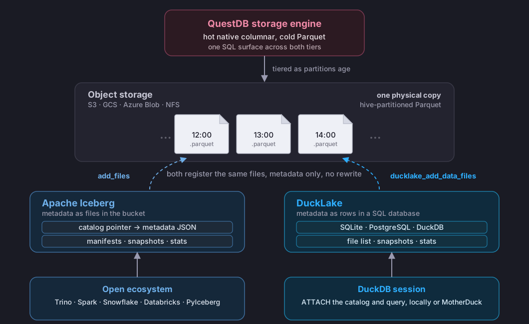
Iceberg registers the same files with add_files for reach across the
lakehouse, and DuckLake attaches them with ducklake_add_data_files for a fast
single-node session.
Storage policies and cold storage are QuestDB Enterprise features. In QuestDB
OSS you can convert partitions to Parquet manually with
ALTER TABLE ... CONVERT PARTITION ... TO PARQUET, or create the table with
FORMAT PARQUET. See the Parquet concept page.
Notebooks, and coding agents that can drive them
The Web Console moves to 2.0 and is no longer a single editor.
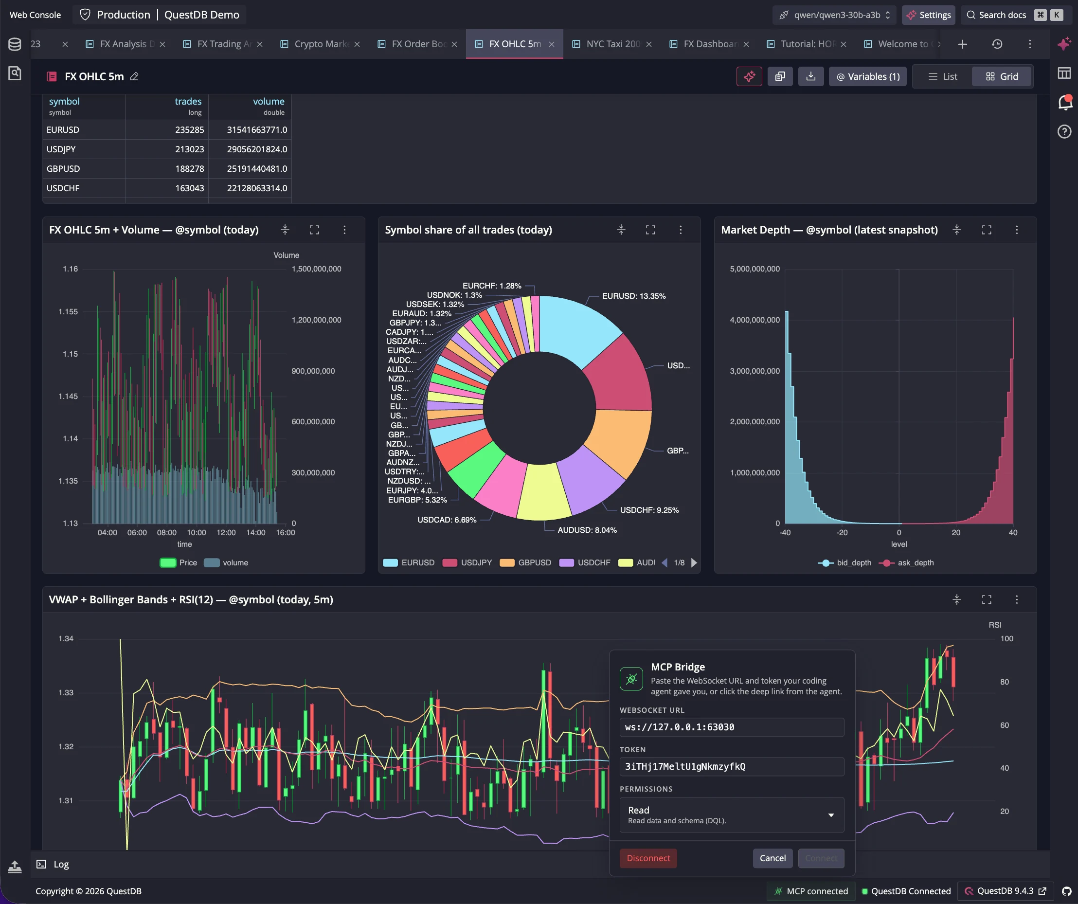
Notebooks mix SQL, markdown and chart cells in one place. Charts render with ECharts and can work out what to plot from the result, cells rearrange into a grid, and a query cell can be turned into a live chart that refreshes itself. Notebooks are stored in your browser, so they survive a reload.
Coding agents can drive that surface. The QuestDB MCP relays Claude Code, Codex, Cursor or any other MCP client to your open console tab. The agent reads your schema, runs SQL, and builds cells and charts in the same notebook you are looking at, so you watch it work and can edit alongside it.
Everything the agent does runs in your browser against the session you already have open, so it never gets your database credentials. Pairing goes through a consent dialog naming what is connecting and what it can do, permissions start read-only, and anything it cannot prove is a read is refused.
The covering index gets its parallel decode
9.4.0 introduced INDEX TYPE POSTING with an optional INCLUDE (...) covering
sidecar, and shipped with a warning: on some workloads the covering plan was
slower than an ordinary scan, and a follow-up would close the gap.
This is that follow-up. Covered column decode now runs across worker threads instead of a single one. Warm JMH, 20M rows, 8 workers, 10% selectivity:
| Query shape | Before | After | Speedup |
|---|---|---|---|
sum | 7.26 ms | 2.15 ms | 3.4x |
| Multi-aggregate | 6.76 ms | 2.25 ms | 3.0x |
first/last | 7.61 ms | 2.08 ms | 3.7x |
| Residual filter | 10.42 ms | 3.04 ms | 3.4x |
| Keyed GROUP BY | 27.06 ms | 7.12 ms | 3.8x |
The number that matters for cold storage is bytes rather than milliseconds. The covering plan reads 1.2x to 4.3x fewer bytes off the device than a full scan, and unlike a scan, that gap widens as the filter gets more selective. On a local NVMe the CPU cost still dominates; on object storage the bytes are the whole story.
Whether it beats a plain scan is a selectivity question: aggregations win below
roughly 5%, keyed GROUP BY below 2%. EXPLAIN tells you which plan you got, and
/*+ no_covering */ opts a query out.
New SQL features
SHOW CREATE DATABASE dumps
the DDL for every table, view and materialized view, one statement per row and
ordered so that replaying them top to bottom works. It is the pg_dump --schema-only you could never run against QuestDB.
QuestDB Enterprise adds users, groups, service accounts and grants to the dump.
Numeric comparisons against a scalar sub-query, so a threshold can be computed inline rather than in two round trips:
SELECT * FROM tradesWHERE price > (SELECT avg(price) FROM trades WHERE timestamp IN '$today');
New functions: the
kurtosis() and
skewness()
aggregates, and
is_end_of_month().
Operations
A handful of changes aimed at whoever runs QuestDB rather than queries it.
Per-query memory limits. You can now cap how much memory a single query is allowed to allocate, with separate caps for materialized view refreshes and WAL apply. All three are off by default, so nothing changes when you upgrade, and all three can be changed without a restart:
cairo.query.memory.limit.bytescairo.mat.view.refresh.memory.limit.bytescairo.wal.apply.memory.limit.bytes
A query that goes over its limit fails, naming itself in the error, while
everything else carries on. query_activity gains memory_used and
memory_limit columns so you can watch a query approaching the line before it
crosses it.
Queries stop when the client goes away. They did not before. A client that
disconnected mid-query left the query running until it hit query.timeout,
holding a connection and a worker for as long as it took. The server now notices
the disconnect and stops the query.
ALTER TABLE ... REBASE WAL
rebuilds a table under a fresh sequencer while
keeping all of its data. It is a recovery tool for a table whose transaction log
has grown unmanageable or gone bad, and for re-baselining a table for
replication.
Restoring a snapshot is faster on tables with many Parquet partitions, and most of all on object or network storage.
Performance and breaking changes
The two big performance stories in this release are QWP and the covering index decode, and both are above. The rest is spread across sorting, partition pruning, window queries and memory use, and it is itemised in the release notes rather than here.
The breaking changes are a handful, mostly in the PostgreSQL catalogue and in two config keys that no longer do anything. If you point PostgreSQL tooling at QuestDB or validate your config strictly, read those before you upgrade. Both lists are in the 10.0.0 release notes on GitHub.
Bug fixes, and the fuzzer behind them
9.4.1 introduced a SQL query fuzzer that generates random query shapes and checks the results the engine returns for them. Together with stricter default assertions in the test framework, it surfaced more than 60 latent correctness and resource-leak bugs on its first pass, in an engine that already carried close to a million lines of test code. Those bugs had been shipping quietly for a long time, and they were fixed before 10.0 rather than after it.
The fuzzer has since grown cursor self-consistency checks and fault injection,
so it now also asks whether a cursor yields the same rows when it is re-read,
and whether the engine survives an allocation failure part-way through a query.
ASOF and LT join fuzzing covers multi-column ON clauses. All of it runs
continuously rather than only before a release.
That is where the long tail of fixes in this release comes from: the posting and covering index, Parquet reads and conversion, the WAL apply path, materialized view refresh, and the SQL planner. The full list is on the release notes page.
Getting 10.0
docker pull questdb/questdb:10.0.0
Or download QuestDB directly. The full changelog is on GitHub.
QWP is new, and we want to know how it behaves outside our own tests. If you try it, tell us where it holds up and where it does not. Find us on Slack or Discourse, or try it on the live demo.
QuestDB Enterprise 4.0, with cold storage, ships in the next few days. Self-managed enterprise customers will find the binaries at the usual download location. BYOC enterprise customers will be contacted for upgrading.
Not on QuestDB Enterprise yet? Learn more about QuestDB Enterprise and BYOC, or contact the QuestDB team for a conversation or a demo.