Market data replay for backtesting: a full day of US equities from QuestDB
A full trading day of US equities, 354 million top-of-book events, streamed back from QuestDB as Arrow. In strict time order the client peaks at 194 MiB; parallel connections reach 14 Gb/s, using more memory as more results arrive at once. Code, commands and hardware included so you can rerun it.



A backtest only gives an honest answer if the past arrives in the order it happened, every quote and trade fed to the same code that will later run live. That makes replay the job a tick store is judged on.
kdb+ built much of its reputation on that job, and its license includes a DeWitt clause, so you can't publish your own kdb+ benchmarks.
What we can show you is how fast QuestDB does it. Below is a full day of every US equity, replayed out of QuestDB as fast as it goes, with the code, the commands and the hardware, so you can rerun it on your own machines and against whatever you run today.
The data comes from Databento's EQUS.MINI, loaded as in our
previous post: 354 million
top-of-book events and 7.5 million trades, 57.6 GB once decoded into Arrow.
- Strict order: about two minutes for the whole day, at 3.5 to 3.8 Gb/s
- Eight connections per table: 32.5 seconds, at 14.2 Gb/s
- Client memory: 194 MiB at peak, about half of it the idle Python process
- One symbol, NVDA: 5.6 to 6.0 seconds end to end, filter included
Replaying one full trading day. Grey bars ran on the database host, with no network.
of Arrow in one full replay
peak client memory, strict order
network link the parallel run filled
The replay works the same on QuestDB open source and QuestDB Enterprise, and the code is in our blog-examples repository.
One trading day of US equities top of book, in one table
Databento's EQUS.MINI blends feeds from US exchanges
and alternative trading systems into one composite best bid and offer per
stock, plus the trades. We loaded two of its schemas for October 27th, 2026:
mbp-1, every change to the top of book, into equs_all_orderbook, and
trades into equs_all_trades. mbp-1 also carries the trade events, so the
order book table on its own is one complete, ordered stream of quotes and
trades.
| Table | Rows | Symbols | On disk |
|---|---|---|---|
equs_all_orderbook | 353,657,441 | 12,684 | 79.2 GB |
equs_all_trades | 7,544,547 | 9,802 | 0.6 GB |
The session runs from 04:00 to 20:00 New York time, but the day isn't even. Regular hours, 09:30 to 16:00, hold 98% of the book events:
Top-of-book events per 5 minutes, Databento EQUS.MINI, Tuesday 2026-10-27, every US equity
of events in regular hours
events in the busiest second
events in the last minute before the close
The busiest second of the day carried 206,101 book events, and the last minute before the close carried 2.5 million. Those are the moments a backtest cares most about, and the ones a sampled or bar-based dataset smooths away.
Both tables come from the
Databento connector in Historical mode,
which is a QuestDB Enterprise feature. The
previous post covers the
connector and the table layout, and the example repository has a
backfill_day.py script that loads a day for NVDA and AAPL, or every symbol
with --all-symbols. On QuestDB open source, load the data with the
Databento Python guide instead, and the
replay below works unchanged.
Every row is wide: 18 columns, four of them arrays.
CREATE TABLE equs_all_orderbook (dataset SYMBOL, -- EQUS.MINIsymbol SYMBOL CAPACITY 16384, -- NVDA, AAPL, ... 12,684 of thempublisher_id INT, -- venue the record came frominstrument_id LONG,ts_event TIMESTAMP_NS, -- when the venue saw the eventprice DOUBLE,size LONG,action SYMBOL, -- A add, C cancel, T trade, ...side SYMBOL, -- B bid, A ask, N noneflags SHORT,depth SHORT,ts_recv TIMESTAMP_NS, -- when Databento received itts_in_delta LONG,sequence LONG,bids DOUBLE[][], -- [[prices], [sizes]], best level firstasks DOUBLE[][],bid_ct DOUBLE[], -- orders at each bid levelask_ct DOUBLE[]) TIMESTAMP(ts_recv) PARTITION BY DAY WAL;
This is what the replay streams back. The first NVDA events after the 09:30 open, in the Web Console, with 8 of those 18 columns:
SELECT ts_recv, symbol, action, side, price, size, bids, asksFROM equs_all_orderbookWHERE symbol = 'NVDA'AND ts_recv IN '2026-10-27T13:30:00Z;1s'LIMIT 8;
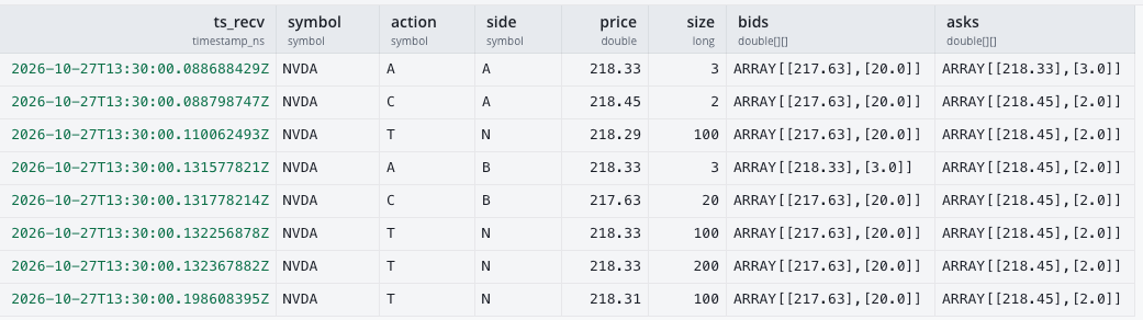
Each row is one event, and bids and asks hold the top of the book right
after it: [[217.63], [20.0]] is 20 shares bid at 217.63. Each array has one
level because mbp-1 is top of book only. A deeper schema such as mbp-10
uses the same columns with more levels, and wider rows.
How the replay streams from QuestDB: Arrow batches over QWP
The replay script, replay.py, uses the
QuestDB Python client, which reads
over QWP, QuestDB's binary protocol
over WebSocket. Results come back as a stream of
Apache Arrow record batches of up to 16,384 rows
each, and the loop at the heart of the script hands each one to the consumer
as it arrives:
with reader.query(sql, reset_symbol_dict=False) as result:for batch in result.iter_arrow():timestamps = to_ns(batch.column("ts_recv"))out_of_order += np.count_nonzero(np.diff(timestamps) < 0)publish(table, batch)
publish() is where your consumer goes: a strategy, a Kafka producer, an order
book rebuild. In the runs below it's empty, so they measure reading. Whatever
you put there sets the pace, and a slow consumer slows its connection down
through QWP's flow control rather than piling batches up in memory. Once
publish() returns, the batch is released, which is why the client's memory
depends on how many connections are open, not on how many rows a query
returns. The out_of_order counter checks the ordering on every batch, and it
was zero in every run.
Why the day is split into a few queries
In principle the whole day is one query: SELECT * FROM equs_all_orderbook,
streamed in timestamp order. In practice every query has to finish within the
server's query.timeout, 60 seconds by default, and a strict replay of the
book takes two minutes or more. So the script cuts each table into consecutive
time ranges with about the same number of rows, using per-minute counts from
QuestDB:
SELECT ts_recv minute, count() rowsFROM equs_all_orderbookSAMPLE BY 1m;
Each connection gets one range, split further only so that no single query exceeds 100 million rows. In strict order the book becomes four queries of about 88 million rows, read one after another on the same connection. The split has no other purpose, and the per-query overhead is negligible.
As of the writing of this post, a per-query timeout for QWP is in progress (see questdb/questdb#7768). Once it ships in the server and the Python client, a strict replay won't need splitting at all.
Strict-order replay: 354 million book events at up to 3.8 Gb/s
By default the example script opens one QuestDB connection per table and sends
its queries one after another. QuestDB returns each query's rows in ts_recv
order, so the table arrives in strict order:
export QDB_CLIENT_CONF='wss::addr=<server>:9000;token=<token>;'python3 replay.py equs_all_orderbook equs_all_trades
equs_all_orderbook: 353,657,441 rows, 0 out of order, 129.0s, 2,742,501 rows/s, 441.6 MB/sequs_all_trades: 7,544,547 rows, 0 out of order, 1.1s, 6,575,707 rows/s, 534.3 MB/sReplayed 361,201,988 rows over 2 connection(s) in 129.0s (2,801,006 rows/s)
Across runs on different days, the order book took between 119.2 and 130.4 seconds, which is 3.5 to 3.8 Gb/s. The trades table finishes in about a second on its own connection while the book carries on.
On the server this used 1.2 of its 32 cores, almost all of it in one network thread. With one connection per table, strict order can't use more than that, and that one thread is the limit. Running the client on the database host doesn't lift it either: strict order took 117.6 to 129.9 seconds there.
Why Gb/s and not rows per second
These rows are wide, about 160 bytes each once decoded into Arrow. The same machinery moves a narrow five-column trades table at 220 million rows a second. Rows per second mostly measures how wide the rows are. Gigabits per second, counted as the decoded Arrow bytes handed to the consumer, is the figure that carries over to your own schema, so it's the one we quote throughout.
Client memory stays flat while 57.6 GB streams through
The replay never holds the day, so the client's memory tracks the number of open connections, not the amount of data:
| Run | Arrow streamed | Peak client memory (RSS) |
|---|---|---|
| Strict order, 2 connections | About 57.6 GB | 194 MiB |
| Parallel, 10 connections | About 57.6 GB | 535 MiB |
A Python process with the client libraries loaded sits at about 100 MiB before it receives anything, so strict order added under 100 MiB on top of that while reading the whole day. A table ten times larger should need the same.
On the server, used memory stayed between 1.5 and 1.8 GB for the whole run, and the page cache sat flat at 78.7 GB because the day was already in it.
Parallel replay: 14.2 Gb/s, until the network runs out
Not every replay needs global order. Fitting a model per time window, checking
features range by range, or warming a cache over a whole day only need each
range in order internally. For those, the example script's --connections
option opens that many QuestDB connections per table and gives each one an
equal share of the day to query. QuestDB serves the queries side by side:
python3 replay.py equs_all_orderbook equs_all_trades --connections 8
equs_all_orderbook: 353,657,441 rows, 0 out of order, 32.5s, 10,882,357 rows/s, 1,752.3 MB/sequs_all_trades: 7,544,547 rows, 0 out of order, 1.1s, 6,975,148 rows/s, 566.7 MB/sReplayed 361,201,988 rows over 10 connection(s) in 32.5s (11,114,510 rows/s)
Both tables in 32.5 seconds, about 11 million rows a second and 14.2 Gb/s of decoded Arrow. Rows are in order within each connection's share, which is what the zero counts, and not across shares. We kept it that way on purpose: putting the shares back in order would mean buffering them, and the point of this mode is speed.
The limit here is the network. Arrow takes more room in memory than on the wire, so the 14.2 Gb/s the client decoded crossed the network as 12.2 Gb/s on average, peaking at 12.5. That's the ceiling: the server is rated at 12.5 Gbps, and the client at up to 12.5 Gbps as a burst above a lower baseline. QuestDB used 8.8 of its 32 cores to get there.
Removing the network: 27 Gb/s on the database host
To see what's behind that ceiling, we ran the client on the server itself,
connecting to localhost and pinned with taskset to cores away from
QuestDB's threads:
| Run, connections per table | Time | Rows/s | Decoded throughput |
|---|---|---|---|
| Over the network, 8 | 32.5 s | 11.11M | 14.2 Gb/s |
| On the server, 8 | 18.7 s | 19.36M | 24.6 Gb/s |
| On the server, 16 | 17.0 s | 21.19M | 27.1 Gb/s |
With the same eight connections, taking the network away made the replay 74% faster. Doubling to 16 added about 10% more, at which point one Python process serves every connection and the client shares the server's CPUs with TLS and loopback copies. These are ceilings, not deployment figures, since nobody runs a backtest on the database host. They show how much room QuestDB has before it becomes the limit.
Replaying one symbol in order: NVDA end to end
A backtest on a single stock doesn't need the other 12,683 symbols. The
script's --symbol option adds symbol = 'NVDA' to every query's filter, and
QuestDB still returns the rows in timestamp order:
python3 replay.py equs_all_orderbook equs_all_trades --symbol NVDA
equs_all_orderbook: 1,382,513 rows, 0 out of order, 6.0s, 229,980 rows/s, 36.8 MB/sequs_all_trades: 29,879 rows, 0 out of order, 0.1s, 268,773 rows/s, 21.5 MB/sReplayed 1,412,392 rows over 2 connection(s) in 6.0s (234,950 rows/s)
Those 5.6 to 6.0 seconds across runs are end to end: QuestDB finds NVDA's
rows, 0.4% of the day's 354 million, and streams them as it finds them, while
the client receives and checks every batch. Those rows are scattered across
the whole day's files, and reading them from all over the day is what takes
the time. With --connections 8, the script splits NVDA's rows equally across
eight connections, and they arrive in 0.9 seconds, in order within each
connection's share.
Where these replay numbers stop: page cache, consumers and book depth
Every figure above comes from the same setup, and a few things would change them:
- The day was in memory. The server had 78.7 GB of page cache holding the whole day, so no run read from disk. A server that can't cache the day reads part of it from storage, and these numbers don't apply.
publish()was empty. A consumer that does per-row work in Python, or buffers the day, will be slower and use more memory. The replay will wait for it.- Top of book only. One level per side. A deeper book such as
mbp-10makes every row bigger, so Gb/s should stay about the same while fewer rows arrive each second. - Tables are independent. With two tables in strict order, each arrives in
order on its own. Because
mbp-1already includes trades, the order book table is the single merged stream here. For other datasets, a merge of two streams on the timestamp belongs in the consumer.
Your numbers will differ with hardware, network and schema, which is why everything is published.
Run the replay on your own hardware
The runs above used an EC2 m7a.8xlarge for QuestDB and an m7a.2xlarge client in the same availability zone. To run the replay on your own hardware, the example repository has the script and every command, from loading the day to the one-symbol runs. It works with QuestDB open source 10.0 or later and QuestDB Enterprise 4.0 or later. Loading the data through the Databento connector needs QuestDB Enterprise; on open source, load it with the Databento Python guide.
If you have a kdb+ estate, the comparison we can't publish is one you can run yourself: the same day, the same consumer, your tickerplant log or HDB on one side and this script on the other. The QuestDB vs kdb+ page covers the rest of the architecture. Getting the data out fast is also what feeds transaction cost analysis in Polars, and the Arrow egress benchmark compares the same read path with ClickHouse and TimescaleDB. If you rerun this, tell us what you measured on the community forum.