Transaction Cost Analysis with QuestDB and Polars: VWAP, Slippage and Markout

Last updated: 20 July 2026.

Every trading desk eventually asks the same question about its executions: did we pay a fair price, or did the market see us coming? Transaction cost analysis (TCA) is how you answer it. You compare each fill against benchmarks like the arrival price and the interval VWAP, then you watch what the market did in the seconds and minutes after you traded. If prices keep running away from your fills, you're being adversely selected, and that costs real money at any size.

The tooling for this usually lives in expensive, specialised systems, which is a shame, because the computation itself is a handful of time-series queries over trades and quotes. So let's build a working TCA pipeline from scratch, with three open tools:

• QuestDB stores the ticks and does the time-series heavy lifting in SQL: interval VWAPs, point-in-time joins between fills and quotes, markout curves at a dozen horizons.
• ConnectorX pulls query results into Python in parallel and hands them over as Arrow, so there's no row-by-row cursor sitting between your database and your dataframe.
• Polars does the dataframe work: percentiles, groupings, the summary tables you'd actually show a desk head.

We'll capture live crypto market data, simulate a TWAP execution against it, then measure what that execution cost, the way a real desk would. Everything runs on a laptop, and we ran every query below on live data before publishing.

Step 1: set up QuestDB and capture live ticks

Start QuestDB and install the Python pieces:

docker run -d --name questdb -p 9000:9000 -p 9009:9009 -p 8812:8812 \
  questdb/questdb:latest

pip install cryptofeed questdb polars pyarrow connectorx

One environment note before anything else: if your Python is an x86 build running under Rosetta on an Apple Silicon Mac, install polars[rtcompat] instead of polars. Rosetta doesn't translate AVX instructions, so stock Polars warns about missing CPU features on import and is liable to crash. We hit this on our own machine; the rtcompat build runs fine.

Create the three tables we need. Open the web console at localhost:9000 and run:

CREATE TABLE IF NOT EXISTS trades (
    ts TIMESTAMP,
    symbol SYMBOL,
    side SYMBOL,
    price DOUBLE,
    amount DOUBLE
) TIMESTAMP(ts) PARTITION BY DAY WAL
DEDUP UPSERT KEYS(ts, symbol);

CREATE TABLE IF NOT EXISTS quotes (
    ts TIMESTAMP,
    symbol SYMBOL,
    bid DOUBLE,
    ask DOUBLE
) TIMESTAMP(ts) PARTITION BY DAY WAL;

CREATE TABLE IF NOT EXISTS fills (
    ts TIMESTAMP,
    symbol SYMBOL,
    side SYMBOL,
    price DOUBLE,
    qty DOUBLE
) TIMESTAMP(ts) PARTITION BY DAY WAL;

trades holds every trade that happens on the exchange, quotes tracks the best bid and ask over time, and fills will hold our own executions. On a real desk fills is your OMS blotter export; here we'll generate it.

Now capture live data with cryptofeed, which streams normalised trades and order books from most major exchanges. The script below writes every trade and every top-of-book update into QuestDB over ILP via HTTP, the ingestion path every QuestDB accepts today:

import os
import certifi
os.environ['SSL_CERT_FILE'] = certifi.where()  # macOS: Homebrew Python lacks system CAs

from cryptofeed import FeedHandler
from cryptofeed.exchanges import OKX
from cryptofeed.defines import TRADES, L2_BOOK
from questdb.ingress import Sender, TimestampNanos

conf = ("http::addr=localhost:9000;"
        "auto_flush_rows=500;auto_flush_interval=1000;")
sender = Sender.from_conf(conf)
sender.establish()

async def trade_cb(t, receipt_timestamp):
    sender.row(
        'trades',
        symbols={'symbol': t.symbol, 'side': t.side},
        columns={'price': float(t.price), 'amount': float(t.amount)},
        at=TimestampNanos(int(t.timestamp * 1e9))
    )

async def book_cb(book, receipt_timestamp):
    best_bid = max(book.book['bid'].keys())
    best_ask = min(book.book['ask'].keys())
    sender.row(
        'quotes',
        symbols={'symbol': book.symbol},
        columns={'bid': float(best_bid), 'ask': float(best_ask)},
        at=TimestampNanos(int(book.timestamp * 1e9))
    )

f = FeedHandler()
f.add_feed(OKX(
    symbols=['BTC-USDT'],
    channels=[TRADES, L2_BOOK],
    callbacks={TRADES: trade_cb, L2_BOOK: book_cb}
))
f.run()

Let it run while you read. Half an hour of BTC-USDT gets you tens of thousands of trades and a few hundred thousand quote updates, plenty for what we're doing. Here's a quick sanity check that the microstructure looks right:

SELECT ts, avg(spread(bid, ask) / mid(bid, ask)) * 10000 AS spread_bps
FROM quotes
WHERE symbol = 'BTC-USDT' AND ts IN '$today'
SAMPLE BY 1m;

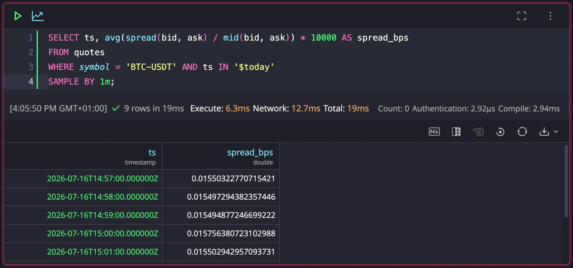
The screenshots in this post are notebook cells in the QuestDB web console, another 10.0 addition: SQL, results and charts side by side with markdown notes, no extra tooling. As for the query itself, spread() and mid() are built-in functions, and SAMPLE BY 1m is QuestDB's native way to bucket a query by time.

Step 2: simulate an execution

First we need an execution to analyse, so let's simulate one: a TWAP order that buys the same amount of BTC every 30 seconds, paying the ask each time. One INSERT builds the whole blotter from the captured quotes:

INSERT INTO fills
SELECT ts, symbol, 'buy', fill_price, 0.05
FROM (
    SELECT ts, symbol, last(ask) AS fill_price
    FROM quotes
    WHERE symbol = 'BTC-USDT' AND ts IN '$today'
    SAMPLE BY 30s
);

Each row is one buy of 0.05 BTC. The timestamp is when the buy was scheduled, and the price is the last ask in that 30-second window, when it filled. This is a deliberately bad algo: it pays the spread on every buy and trades on a fixed clock, so its costs will be easy to see in the analysis. If you have a real blotter, load it into fills instead and everything from here on applies unchanged.

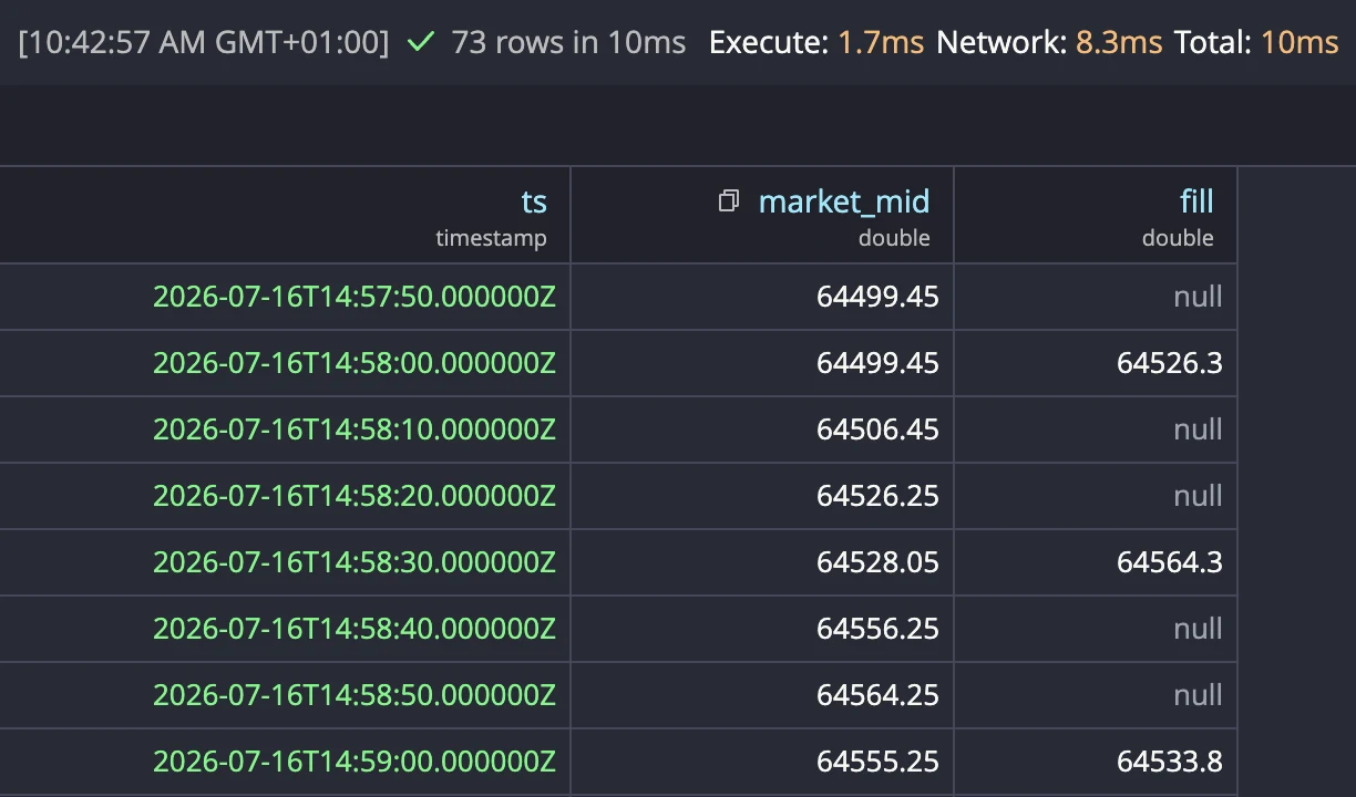
It helps to see what the algo actually did before measuring anything. One more notebook cell charts the fills on top of the market mid:

SELECT q.ts, mid(q.bid, q.ask) AS market_mid, f.price AS fill
FROM (
    SELECT ts, symbol, last(bid) AS bid, last(ask) AS ask
    FROM quotes
    WHERE symbol = 'BTC-USDT' AND ts IN '$today'
    SAMPLE BY 10s
) q
LEFT JOIN fills f ON q.ts = f.ts;

The two timestamps land on aligned bucket starts, so every 10-second row shows the mid, and a fill price appears wherever a buy landed:

Step 3: measure the costs in SQL

Did we beat VWAP?

The first question every TCA report answers: how did our average fill price compare with the market's volume-weighted average price over the same window? QuestDB has a built-in vwap() aggregate, but it averages the raw trade price, and our own docs steer you away from it. The benchmark a desk uses is the running VWAP over the typical price (high + low + close) / 3: downsample the trades into ten-second candles, then take a cumulative volume-weighted average across them, all in one query. The VWAP cookbook recipe has the canonical form:

WITH candles AS (
    SELECT ts,
        max(price) AS high, min(price) AS low, last(price) AS close,
        sum(amount) AS volume
    FROM trades
    WHERE symbol = 'BTC-USDT' AND ts IN '$today'
    SAMPLE BY 10s
)
SELECT ts, close AS price,
    sum((high + low + close) / 3 * volume) OVER (ORDER BY ts CUMULATIVE)
    / sum(volume) OVER (ORDER BY ts CUMULATIVE) AS vwap
FROM candles;

Comparing it against our own fills is one more query:

WITH ours AS (
    SELECT sum(price * qty) / sum(qty) AS avg_fill
    FROM fills
    WHERE ts IN '$today'
),
candles AS (
    SELECT (max(price) + min(price) + last(price)) / 3 AS typical,
           sum(amount) AS volume
    FROM trades
    WHERE symbol = 'BTC-USDT' AND ts IN '$today'
    SAMPLE BY 10s
),
mkt AS (
    SELECT sum(typical * volume) / sum(volume) AS market_vwap
    FROM candles
)
SELECT avg_fill, market_vwap,
       (avg_fill - market_vwap) / market_vwap * 10000 AS vs_vwap_bps
FROM ours CROSS JOIN mkt;

Positive vs_vwap_bps means we paid more than the market average. A spread-crossing TWAP should land at a small positive number: roughly the average half-spread, plus whatever the market drifted against us.

Arrival slippage, fill by fill

VWAP only tells you so much, though. The benchmark desks take more seriously is the arrival price: where the mid was when each buy was scheduled. Our fills carry exactly that timestamp, so this is a point-in-time lookup from every fill into the quotes stream, which is what ASOF JOIN is for. It matches each fill with the most recent quote at or before the fill's timestamp. No bucketing, no correlated subqueries:

SELECT
    f.ts,
    f.price AS fill_price,
    mid(q.bid, q.ask) AS mid_at_fill,
    spread(q.bid, q.ask) AS spread_at_fill,
    (f.price - mid(q.bid, q.ask)) / mid(q.bid, q.ask) * 10000 AS slippage_bps
FROM fills f
ASOF JOIN quotes q ON (symbol)
WHERE f.ts IN '$today';

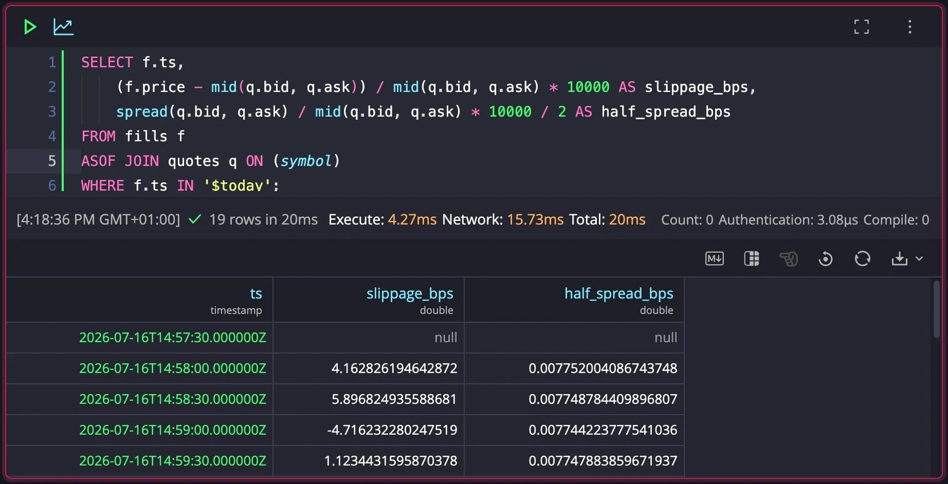
For buys, positive slippage is cost, and there are two things inside it: the half-spread you pay for crossing, plus whatever the market moved between the buy being scheduled and it filling. On a book as tight as BTC-USDT the spread part is nearly invisible (hundredths of a basis point in our run), so what you're really looking at is drift. Symmetric noise around zero is what a healthy schedule looks like. A mean that stays positive says the algo keeps buying into rising prices. Note the null on the first fill, which landed before our first captured quote: ASOF JOIN reports no match rather than inventing one. For sells you flip the sign convention, a one-line CASE on side.

You can try this without installing anything: run the FX version on the live demo: the same ASOF JOIN over fx_trades and market_data, with the buy and sell sign conventions wired in, against yesterday's data.

The markout curve

Slippage tells you what you paid at the moment of execution. Markout tells you what happened next, which is where adverse selection shows up. For each fill we want the mid at a grid of offsets around the execution: 30 seconds before, at the fill, 30 seconds after, and so on out to five minutes.

In most databases this query is painful, because it's an ASOF join repeated at many time offsets per row. QuestDB has a construct for exactly this, HORIZON JOIN, and it evaluates the whole grid in one parallel pass:

SELECT
    h.offset / 1000000 AS horizon_sec,
    avg((mid(m.bid, m.ask) - f.price) / f.price * 10000) AS avg_markout_bps
FROM fills f
HORIZON JOIN quotes m ON (symbol)
    RANGE FROM -30s TO 5m STEP 30s AS h
WHERE f.ts IN '$today'
GROUP BY horizon_sec
ORDER BY horizon_sec;

One unit detail we hit running this ourselves: h.offset comes back in the table's timestamp precision. Our tables use default microsecond timestamps, hence the division by 1,000,000. On nanosecond tables divide by 1,000,000,000 instead, or the whole curve silently collapses into the zero bucket.

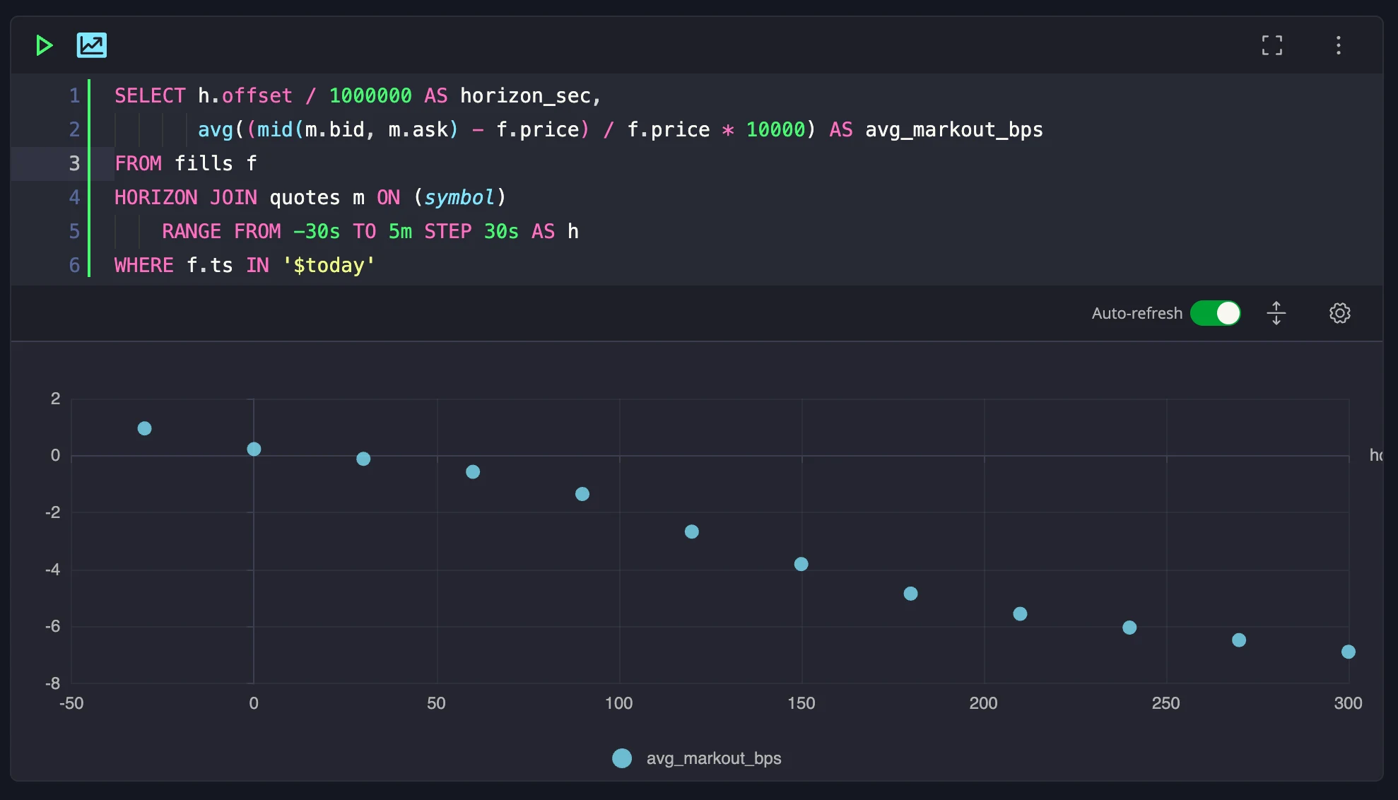
Reading the curve for a buy order:

• At zero, the markout is your slippage with the sign flipped.
• Rising after zero: the market kept going up after the buys, so the fills look good in hindsight.
• Falling after zero: prices came back after the buys. A curve that keeps ending negative means the execution is losing money to timing.
• Before zero: the run-up into each fill. A steep climb means the schedule buys after prices rise.

The same query runs on live data with no setup: open the FX markout on the demo, a HORIZON JOIN over fx_trades broken out by venue, counterparty and horizon.

One caveat: our fills are simulated, so none of this drift is impact we caused. BTC simply fell during that stretch of the session. On a real blotter the same shape would be worth investigating. The capital markets cookbook has more recipes built on the same joins: slippage aggregation, implementation shortfall and last-look detection.

Step 4: hand off to Polars with ConnectorX

We could compute everything below in SQL too, but sooner or later the analysis moves to a notebook, so let's get the per-fill results into a dataframe.

We use ConnectorX for the Polars integration. It reads from QuestDB over the PostgreSQL wire protocol on port 8812.

import polars as pl

URI = "redshift://admin:quest@localhost:8812/qdb"

FILLS_SQL = """
SELECT
    f.ts,
    f.price AS fill_price,
    f.qty,
    mid(q.bid, q.ask) AS mid_at_fill,
    spread(q.bid, q.ask) AS spread_at_fill,
    (f.price - mid(q.bid, q.ask)) / mid(q.bid, q.ask) * 10000 AS slippage_bps
FROM fills f
ASOF JOIN quotes q ON (symbol)
WHERE f.ts IN '$today'
"""

fills = pl.read_database_uri(query=FILLS_SQL, uri=URI)

ConnectorX reads the result straight into Arrow memory, and on large result sets it partitions the read across threads. From here it's ordinary Polars. The headline numbers:

summary = fills.select(
    pl.len().alias("fills"),
    pl.col("slippage_bps").mean().round(2).alias("mean_bps"),
    pl.col("slippage_bps").median().round(2).alias("median_bps"),
    pl.col("slippage_bps").quantile(0.95).round(2).alias("p95_bps"),
    ((pl.col("slippage_bps") / 1e4) * pl.col("fill_price") * pl.col("qty"))
        .sum().round(2).alias("total_cost_usd"),
)

On our capture session's blotter, that prints:

shape: (1, 5)
┌───────┬──────────┬────────────┬─────────┬────────────────┐
│ fills ┆ mean_bps ┆ median_bps ┆ p95_bps ┆ total_cost_usd │
│ ---   ┆ ---      ┆ ---        ┆ ---     ┆ ---            │
│ u64   ┆ f64      ┆ f64        ┆ f64     ┆ f64            │
╞═══════╪══════════╪════════════╪═════════╪════════════════╡
│ 19    ┆ -0.23    ┆ -1.1       ┆ 5.09    ┆ -1.32          │
└───────┴──────────┴────────────┴─────────┴────────────────┘

Nineteen fills. On average each one landed 0.23 bps below its arrival price, and the whole run came in $1.32 under the arrival benchmark. Prices were falling, so every fill looked cheap against the mid from 30 seconds earlier, even though waiting would have been cheaper still.

The same numbers grouped by hour:

by_hour = (
    fills
    .with_columns(pl.col("ts").dt.hour().alias("hour"))
    .group_by("hour")
    .agg(
        pl.len().alias("fills"),
        pl.col("slippage_bps").mean().round(2).alias("mean_slippage_bps"),
        (pl.col("spread_at_fill") / pl.col("mid_at_fill") * 1e4 / 2)
            .mean().round(2).alias("half_spread_bps"),
    )
    .sort("hour")
)

shape: (2, 4)
┌──────┬───────┬───────────────────┬─────────────────┐
│ hour ┆ fills ┆ mean_slippage_bps ┆ half_spread_bps │
│ ---  ┆ ---   ┆ ---               ┆ ---             │
│ i8   ┆ u64   ┆ f64               ┆ f64             │
╞══════╪═══════╪═══════════════════╪═════════════════╡
│ 14   ┆ 5     ┆ 1.62              ┆ 0.01            │
│ 15   ┆ 14    ┆ -0.75             ┆ 0.01            │
└──────┴───────┴───────────────────┴─────────────────┘

In the first hour prices were rising and the fills averaged +1.62 bps of slippage; in the second hour prices fell and the average went negative. The half-spread column barely registers, so nearly all of the cost is price movement. If one hour is consistently expensive, that is where the algo should slow down or work orders passively.

Where to take it

That's the whole pipeline: a session of live trades and quotes captured into QuestDB, a simulated TWAP execution, and its costs measured in SQL with VWAP, arrival slippage and markout queries. ConnectorX and Polars took the per-fill results the rest of the way to summary tables.

From here, the next steps are all small ones:

• Replace the simulated blotter with your real one and add venue and counterparty columns; the same queries become an execution scorecard.
• Decompose costs properly with the implementation shortfall recipe, which splits slippage into spread cost, temporary impact and permanent impact.
• Point the capture script at more symbols and let it run; the tables and queries don't change, only the volume does.
• Reuse the pipeline for backtesting: the same trades-and-quotes store that measures yesterday's executions is the input your strategy simulations replay.

If you're coming from the kdb+ world this workflow will feel familiar, and that's deliberate: see how the two systems compare in our QuestDB versus kdb+ breakdown. For the concepts behind the metrics, the glossary covers slippage and market impact estimation, and our order book imbalance analysis post digs further into reading the book itself. And if you'd like to see the queries run before installing anything, every SQL block in this post works against the FX dataset on the live demo with only table and column names swapped.