Which time-series join? ASOF, WINDOW, HORIZON, LT or SPLICE
A plain-language guide to QuestDB's five time-series joins: ASOF, WINDOW, HORIZON, LT and SPLICE, each with a query that runs on the live demo.



A regular SQL join matches rows whose keys are equal. That works for customer
and order IDs, for example, and falls apart for time. A EURUSD trade executed at
14:54:42.340948053 and the nearest quote was published 17 milliseconds
earlier. Join those two tables on trades.timestamp = quotes.timestamp and you
get zero rows, because two independent feeds almost never share a timestamp.
Mismatched clocks are only part of it, though. Even if every timestamp lined up, the questions we ask of time-series data are rarely about a single instant. What was the quote just before this trade? How busy was the book in the five seconds around it? Where was the price a minute after? None of those is an equality. In standard SQL they turn into range predicates, self-joins and correlated subqueries, which are awkward to write and easy to get subtly wrong.
So QuestDB has five joins built on how rows relate in time instead of on
equality. ASOF and LT look back from each row to the latest value before it.
WINDOW looks at everything in a range around it. HORIZON looks at fixed
points before and after it. SPLICE interleaves two series so that each one
looks back at the other. The reference docs cover the
syntax of each. The question I actually get asked is which one to use, and that
depends on what you're trying to find out. WINDOW and HORIZON are easy to
confuse with each other, and LT and SPLICE cover narrower situations than
the other three, so they get the shortest sections.
Every query below runs on the public demo at demo.questdb.com, against the same two tables, so you can see one set of trades answer a different question each time the join changes.
The short version: which time-series join answers which question
| You want to know | Join | You get back |
|---|---|---|
| The latest value at the moment each event happened | ASOF JOIN | One row per event |
| Everything that happened in a time range around each event | WINDOW JOIN | One aggregated row per event |
| The value at fixed offsets before and after each event | HORIZON JOIN | One row per offset, per event or overall |
| The previous value, strictly before each row's timestamp | LT JOIN | One row per event |
| Every change on either of two feeds, with neither in charge | SPLICE JOIN | One row per row of either table |
| The result of a subquery, run once for each outer row | LATERAL JOIN | The subquery's rows |
ASOF JOIN gives you one row from the other table, WINDOW JOIN gives you
an aggregate over many rows from the other table, and HORIZON JOIN gives
you one row from the other table at each of several offsets. Most questions
are one of those three.
The data: FX trades and quotes on the demo
The demo runs a simulated FX market for 30 currency pairs: around 200,000 trades an hour against more than 6 million quotes, about thirty quotes for every trade. Nearly every query here joins the first of these tables to the second, and the demo data schema page documents all of them:
fx_trades: FX executions. Symbol, side, price, quantity, the ECN (the venue) the trade happened on, and a nanosecond timestamp.market_data: order book snapshots for the same pairs, withbest_bidandbest_askat the top of the book and a microsecond timestamp.core_price: the same quotes broken down per ECN. Only theSPLICE JOINexamples use it.
The prices are anchored to reality: the top of the book tracks real reference
rates, synced from Yahoo Finance every few seconds. Everything else is
synthetic. Every size, the per-ECN quotes in core_price, the book levels
beyond the best, the ticks between two syncs and the trades themselves are
generated around that reference. Read the result tables for the shape of what
each join returns, not for any insight into FX markets. The tables also only
keep a few days of history, so every query uses a relative time range like
'$now - 1h..$now'. Your numbers will differ from mine, which are from the
afternoon of September 21st.
All time-series joins need a
designated timestamp on both tables. You
never write the timestamp condition yourself. The join knows which column is
time, and ON (symbol) only says which other columns have to match.
ASOF JOIN: what was the quote when this trade happened?
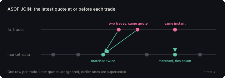
ASOF JOIN takes each row on the left and finds the most recent row on the
right whose timestamp is at or before it. One row in, one row out.
This is the join most people need, most of the time. A trade only makes sense next to the market it happened in:
SELECT t.timestamp, t.side, t.price,m.timestamp AS quote_ts,(m.best_bid + m.best_ask) / 2 AS midFROM fx_trades tASOF JOIN market_data m ON (symbol)WHERE t.symbol = 'EURUSD'AND t.timestamp IN '$now - 1h..$now'LIMIT -5;
| timestamp | side | price | quote_ts | mid |
|---|---|---|---|---|
| 14:54:42.340948053 | buy | 1.1513 | 14:54:42.323945 | 1.1511 |
| 14:54:42.341001570 | buy | 1.1512 | 14:54:42.323945 | 1.1511 |
| 14:54:42.341234503 | buy | 1.1515 | 14:54:42.323945 | 1.1511 |
| 14:54:43.191021280 | sell | 1.1509 | 14:54:43.177697 | 1.1512 |
| 14:54:43.191197265 | sell | 1.1508 | 14:54:43.177697 | 1.1512 |
Three trades within 300 microseconds of each other all pick up the same quote, because it was still the latest one. The trades have nanosecond timestamps and the quotes have microsecond ones. QuestDB aligns them, so there's nothing to cast.
Once every trade carries its mid, the first use case is one avg() away. How
much did I pay over mid, per venue?
WITH priced AS (SELECT t.ecn, t.side, t.price,(m.best_bid + m.best_ask) / 2 AS midFROM fx_trades tASOF JOIN market_data m ON (symbol) TOLERANCE 1sWHERE t.symbol = 'EURUSD'AND t.timestamp IN '$now - 1h..$now')SELECT ecn, count() AS trades,avg(CASE WHEN side = 'buy' THEN 1 ELSE -1 END* (price - mid) / mid * 10000) AS cost_bpsFROM pricedORDER BY cost_bps;
| ecn | trades | cost_bps |
|---|---|---|
| EBS | 6978 | 3.66 |
| Hotspot | 6921 | 3.73 |
| LMAX | 7069 | 3.75 |
| Currenex | 7090 | 3.82 |
Note the TOLERANCE 1s. Without it, ASOF JOIN will happily reach back as far
as it has to: if the quote feed died for ten minutes, every trade in that gap
gets priced against a ten-minute-old quote, and nothing in the result tells you.
With TOLERANCE, a match older than the limit comes back as NULL instead.
There's a whole post on it.
Use ASOF JOIN when each event needs the state of something else at that
moment. Outside finance that's a sensor reading with the calibration that was in
force, a delivery scan with the van's last GPS position, a log line with the
configuration version that was deployed.
Use something else when one row isn't enough. If the question has the word
"average" or "how many" in it, it might be a WINDOW JOIN.
For how ASOF JOIN works under the hood, see
ASOF JOIN, the "do what I mean" of the database world.
WINDOW JOIN: what happened around each trade?
WINDOW JOIN draws a time range around each left row and aggregates every right
row that falls inside it. Still one row out per row in, but now it summarises
many rows from the other table.
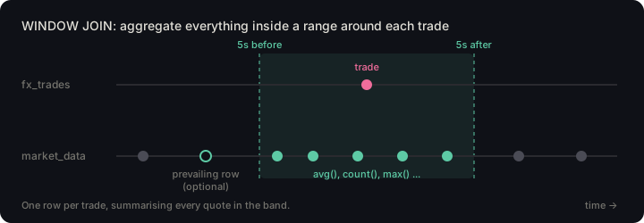
The range can sit anywhere relative to the row: around it, entirely before it,
or entirely after it. And WINDOW JOINs chain, so one query can look at two
different ranges. Did the spread widen after large trades?
SELECT t.timestamp, t.side, t.quantity,avg(b.best_ask - b.best_bid) AS spread_before,avg(a.best_ask - a.best_bid) AS spread_after,count(a.best_bid) AS quotes_afterFROM fx_trades tWINDOW JOIN market_data b ON (t.symbol = b.symbol)RANGE BETWEEN 5 seconds PRECEDING AND 1 microsecond PRECEDINGEXCLUDE PREVAILINGWINDOW JOIN market_data a ON (t.symbol = a.symbol)RANGE BETWEEN 1 microsecond FOLLOWING AND 5 seconds FOLLOWINGEXCLUDE PREVAILINGWHERE t.symbol = 'EURUSD'AND t.timestamp IN '$now - 1h..$now - 1m'AND t.quantity > 500000LIMIT -5;
| timestamp | side | quantity | spread_before | spread_after | quotes_after |
|---|---|---|---|---|---|
| 14:52:25.218 | buy | 594242 | 0.00060 | 0.00042 | 349 |
| 14:52:28.160 | buy | 517782 | 0.00052 | 0.00025 | 337 |
| 14:53:07.513 | buy | 565353 | 0.00047 | 0.00036 | 337 |
| 14:53:07.513 | buy | 763870 | 0.00047 | 0.00036 | 337 |
| 14:53:25.524 | buy | 519662 | 0.00038 | 0.00037 | 250 |
Each spread_after is an average over a few hundred quotes, the count in the
last column.
EXCLUDE PREVAILING. By default a window also includes the last row from before the range starts, the wayASOF JOINwould, so that a quiet window still has a value. That's right for "what was the price during this period" and wrong for "how many quotes arrived", so here it's off.$now - 1mas the upper bound. A trade from three seconds ago doesn't have five seconds of future yet, so itsspread_afterwould be an average over a partial window. Stopping a minute short keeps every window complete.- No
GROUP BY. The aggregates belong to the join, one result per left row. To aggregate those results, wrap the join in a CTE, as in combining joins.
Despite the name, WINDOW JOIN isn't related to window functions. Window
functions (OVER (...)) look at neighbouring rows of the same result set.
WINDOW JOIN looks at rows of a different table that are close in time.
Use WINDOW JOIN when each event needs a summary of what another series was
doing nearby: quote counts, average spread, the max price in the following
minute. For each machine alarm, the average vibration in the 30 seconds before
it. For each deploy, the error count in the 10 minutes after.
Use something else when you want a value at a point instead of over a
range, or when you want that value at several offsets, not over one range.
That's HORIZON JOIN.
How we made WINDOW JOIN parallel and vectorized covers why this runs as fast as it does.
HORIZON JOIN: what happened at fixed offsets before and after each trade?
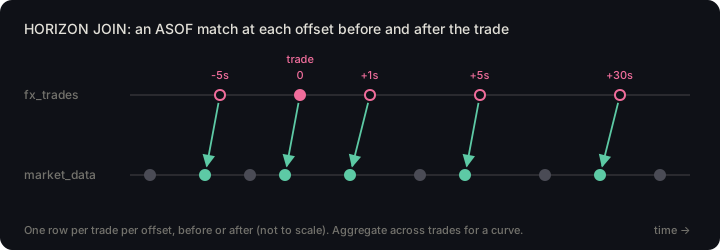
HORIZON JOIN is an ASOF JOIN repeated at several distances from each event.
An offset is one of those distances: a signed duration, measured from the
event's own timestamp. An offset of 5s means "five seconds after this trade",
-5s means five seconds before it, and 0 is the trade itself, which is where a
plain ASOF JOIN would look. For each left row and each offset, the join adds
the offset to the row's timestamp and finds the latest right row at or before
that point.
You give the offsets either as an explicit list, LIST (-5s, 0, 1s, 5s), or as
a grid, RANGE FROM 0s TO 1m STEP 5s, and give the set an alias, usually h.
That alias is a small pseudo-table with two columns: h.offset, the distance,
and h.timestamp, the event's timestamp plus the distance. h.offset is
reported in the left table's timestamp unit, and fx_trades is in nanoseconds,
hence the divisions by a billion below.
On its own the join returns plain rows, one per event per offset, with the
event's columns and the matched right row's columns side by side. Nothing is
aggregated unless you ask for it. Select only h.offset and an avg(), and
the same join collapses thousands of events into one curve.
The textbook use is a markout curve: after I trade, does the market move for me
or against me, and how quickly? The offsets before the trade matter as much. If
the mid was already moving in the five seconds before my fill, somebody knew
something. Positive means the mid is on the favourable side of the trade price.
The SELECT below names only the offset and the side, so every trade in the
hour is rolled into one curve per side:
SELECT h.offset / 1_000_000_000 AS horizon_sec,t.side,count() AS trades,avg(CASE WHEN t.side = 'buy' THEN 1 ELSE -1 END* ((m.best_bid + m.best_ask) / 2 - t.price)/ t.price * 10000) AS markout_bpsFROM fx_trades AS tHORIZON JOIN market_data AS m ON (symbol)LIST (-5s, 0, 1s, 5s, 30s, 1m) AS hWHERE t.symbol = 'EURUSD'AND t.timestamp IN '$now - 1h..$now - 1m'ORDER BY t.side, horizon_sec;
| horizon_sec | side | trades | markout_bps |
|---|---|---|---|
| -5 | buy | 14236 | -3.53 |
| 0 | buy | 14236 | -3.86 |
| 1 | buy | 14236 | -3.88 |
| 5 | buy | 14236 | -3.94 |
| 30 | buy | 14236 | -3.91 |
| 60 | buy | 14236 | -4.04 |
| -5 | sell | 13958 | -3.95 |
| 0 | sell | 13958 | -3.89 |
| 1 | sell | 13958 | -3.93 |
| 5 | sell | 13958 | -3.92 |
| 30 | sell | 13958 | -3.23 |
| 60 | sell | 13958 | -3.07 |
The same twelve numbers as a curve, which is how a markout is usually read:
↑ Higher is better for the trader
Average markout of EURUSD demo trades, one hour on 2026-09-21, 14,236 buys and 13,958 sells
That's 28,194 trades matched at six offsets each, about 169,000 point-in-time lookups, in under 200 ms. The level makes sense: the demo's trades fill against the book, walking past the first level when they're large, so a buy pays the ask or worse and every markout starts a few basis points negative. The flatness is the synthetic part. Generated trades carry no information, so nothing happens to the price after them. On real flow this is where you'd see adverse selection: a curve that keeps sinking after the fill.
WINDOW JOIN vs HORIZON JOIN
These are the two that get mixed up, since both look at the time around an event. They differ in what they measure and in what they return:
WINDOW JOIN | HORIZON JOIN | |
|---|---|---|
| Looks at | every right row inside a range | the latest right row at each offset |
| Aggregates | the rows in the range, always | only if you ask for it |
| Returns | one row per event | one row per offset, per event or overall |
| Answers | the average spread in the 5s after this trade | the mid 5s before and after a trade, on average |
Both can look backwards, forwards or both ways, so direction doesn't tell them apart. If the sentence describing what you want contains "during", it's a window. If it contains "earlier" or "later", it's a horizon.
Use HORIZON JOIN when you're studying the average shape of things around a
kind of event: markouts, whether prices drift ahead of news and how far they
move after it, how long a temperature takes to settle after a valve opens, what
p99 latency looks like 5 minutes before a deploy and 1, 5 and 15 minutes after
it.
Use something else when there's only one offset and it's zero. That's a
plain ASOF JOIN, with none of the restrictions listed further down.
The markout recipe in the cookbook goes
further, and the
transaction cost analysis post
uses HORIZON JOIN from Python.
LT JOIN: the last value strictly before this one (and when lag() is enough)
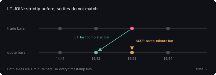
LT JOIN is ASOF JOIN with one change: a right row with exactly the same
timestamp doesn't count. ASOF matches at or before, LT matches before.
On tick data it almost never matters. I ran both joins over an hour of demo trades, 212,129 of them across all 30 symbols, and they picked the same quote every single time. A nanosecond trade clock and a microsecond quote clock don't tie.
And the example you'll usually see for it, joining a table to itself to get the previous row, is easier with a window function:
SELECT timestamp, price,lag(price) OVER (ORDER BY timestamp) AS prev_priceFROM fx_tradesWHERE symbol = 'EURUSD'AND timestamp IN '$now - 1m..$now'LIMIT -5;
But lag() only sees rows of its own result set. It can't reach into another
table, and that's where LT JOIN is the right tool: whenever both sides are
bucketed, because then every timestamp ties.
Build one-minute bars from trades and one-minute bars from quotes, and join them:
WITH trade_bars AS (SELECT timestamp, symbol, last(price) AS trade_closeFROM fx_tradesWHERE symbol = 'EURUSD' AND timestamp IN '$now - 6m..$now'SAMPLE BY 1m),quote_bars AS (SELECT timestamp, symbol,last((best_bid + best_ask) / 2) AS mid_closeFROM market_dataWHERE symbol = 'EURUSD' AND timestamp IN '$now - 6m..$now'SAMPLE BY 1m)SELECT t.timestamp AS bar, t.trade_close,a.timestamp AS asof_bar, a.mid_close AS asof_mid,l.timestamp AS lt_bar, l.mid_close AS lt_midFROM trade_bars tASOF JOIN quote_bars a ON (symbol)LT JOIN quote_bars l ON (symbol);
| bar | trade_close | asof_bar | asof_mid | lt_bar | lt_mid |
|---|---|---|---|---|---|
| 14:41 | 1.1491 | 14:41 | 1.14970 | NULL | NULL |
| 14:42 | 1.1507 | 14:42 | 1.15025 | 14:41 | 1.14970 |
| 14:43 | 1.1546 | 14:43 | 1.15480 | 14:42 | 1.15025 |
| 14:44 | 1.1569 | 14:44 | 1.15740 | 14:43 | 1.15480 |
| 14:45 | 1.1574 | 14:45 | 1.15720 | 14:44 | 1.15740 |
| 14:46 | 1.1526 | 14:46 | 1.15295 | 14:45 | 1.15720 |
| 14:47 | 1.1508 | 14:47 | 1.15050 | 14:46 | 1.15295 |
A bar stamped 14:43 covers 14:43:00 to 14:43:59. Its mid_close is a
value from the end of that minute. ASOF JOIN matches it to the 14:43 trade
bar, which means a strategy reading that row at 14:43:00 would be using a price
it couldn't have known for another 59 seconds. That's look-ahead bias, and it's
how backtests end up better than live trading. LT JOIN returns the 14:42
bar, the last one that had finished.
The first row has no LT match, since nothing came before it. With ASOF that
edge never shows up, because a bar always matches its own minute.
Even on a single table LT JOIN and lag() aren't quite the same. With
duplicate timestamps, lag() steps back one row and may hand you a row from
the same instant, while LT JOIN steps back to the last earlier timestamp.
LT JOIN also accepts TOLERANCE, so "the previous value, but only if it's
recent" is one clause.
Use LT JOIN when both sides share a time grid: bars against bars, hourly
energy usage against hourly prices, daily closes against daily rates.
Use something else when you want the previous row of the same table
(lag()), or when you're joining raw ticks (ASOF JOIN).
SPLICE JOIN: merging two time series when neither one drives
Every join so far has a driver. The left table decides which moments exist, and the right table is looked up at those moments. If the right table changes five times between two left rows, four of those changes never appear in the output.
Sometimes neither side should be in charge. SPLICE JOIN returns a row for
every row of either table, each paired with the prevailing row from the
other side. It's a full outer ASOF JOIN.
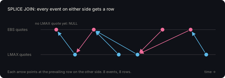
The case for it is comparing two sources of the same thing. Here are EURUSD
bids from two venues. I want to see the gap between them every time either
venue updates:
WITH ebs AS (SELECT timestamp, bid_price FROM core_priceWHERE symbol = 'EURUSD' AND ecn = 'EBS'AND timestamp IN '$now - 2s..$now'),lmax AS (SELECT timestamp, bid_price FROM core_priceWHERE symbol = 'EURUSD' AND ecn = 'LMAX'AND timestamp IN '$now - 2s..$now')SELECT ebs.timestamp AS ebs_ts, lmax.timestamp AS lmax_ts,ebs.bid_price AS ebs_bid, lmax.bid_price AS lmax_bidFROM ebsSPLICE JOIN lmax;
| ebs_ts | lmax_ts | ebs_bid | lmax_bid |
|---|---|---|---|
| ... | |||
| 14:55:06.318979 | 14:55:06.660834 | 1.1526 | 1.1527 |
| 14:55:06.318979 | 14:55:06.672994 | 1.1526 | 1.1527 |
| 14:55:06.318979 | 14:55:06.689447 | 1.1526 | 1.1527 |
| 14:55:06.707103 | 14:55:06.689447 | 1.1527 | 1.1527 |
| 14:55:06.953682 | 14:55:06.689447 | 1.1527 | 1.1527 |
| 14:55:06.970340 | 14:55:06.689447 | 1.1527 | 1.1527 |
| 14:55:07.053136 | 14:55:06.689447 | 1.1527 | 1.1527 |
| 14:55:07.053136 | 14:55:07.071652 | 1.1527 | 1.1527 |
| ... |
Read down the two timestamp columns. In the first three rows the EBS quote
stands still while LMAX ticks three times. Then LMAX stands still while EBS
ticks four times. With ebs ASOF JOIN lmax, those first three rows would be one
row, and two LMAX updates would be gone. The row count tells you which join you
ran: ASOF returns as many rows as the left table, SPLICE returns as many as
both tables together.
The rows I trimmed from the top have NULL on one side. Until the second venue
publishes its first quote inside the time range, there's nothing prevailing to
pair with.
Over a longer range it aggregates like any other query. The same two venues over an hour, counted instead of listed:
WITH ebs AS (SELECT timestamp, bid_price FROM core_priceWHERE symbol = 'EURUSD' AND ecn = 'EBS'AND timestamp IN '$now - 1h..$now'),lmax AS (SELECT timestamp, bid_price FROM core_priceWHERE symbol = 'EURUSD' AND ecn = 'LMAX'AND timestamp IN '$now - 1h..$now')SELECT count() AS events,sum(CASE WHEN ebs.bid_price > lmax.bid_priceTHEN 1 ELSE 0 END) AS ebs_higher,sum(CASE WHEN ebs.bid_price < lmax.bid_priceTHEN 1 ELSE 0 END) AS lmax_higherFROM ebsSPLICE JOIN lmax;
| events | ebs_higher | lmax_higher |
|---|---|---|
| 50668 | 10196 | 10232 |
50,668 events in the hour, the two venues disagreed on about 40% of them, and neither led more often than the other. On simulated data that symmetry is what you'd expect. On real feeds, a lopsided split is how you find the venue that moves first.
Use SPLICE JOIN when you have two streams of equal standing and you care
about every change on both: a primary and a backup price feed, two redundant
sensors on one machine, your own order book against the exchange's.
Use something else when one table is the subject and the other is context.
That's most queries, and that's ASOF JOIN. SPLICE is the one in this list
I'd expect most people never to need, and the one with no tidy workaround when
you do.
LATERAL JOIN: not a time-series join, but it runs them per row
LATERAL JOIN doesn't match on time, so strictly it doesn't belong here. It
earns a section because it's how you run any of the above once per something.
A lateral subquery can see the columns of the row to its left, so it behaves
like a function called for each outer row. The classic use is top-N per group.
And since the subquery is a full query, it can contain its own ASOF JOIN. The
two largest trades per symbol in the last hour, each with the mid at the time:
SELECT s.symbol, big.timestamp, big.side, big.quantity,big.price, big.midFROM (SELECT DISTINCT symbol FROM fx_tradesWHERE timestamp IN '$now - 1h..$now'AND symbol IN ('EURUSD', 'USDJPY', 'GBPUSD')) sJOIN LATERAL (SELECT f.timestamp, f.side, f.quantity, f.price,(m.best_bid + m.best_ask) / 2 AS midFROM fx_trades fASOF JOIN market_data m ON (symbol)WHERE f.symbol = s.symbolAND f.timestamp IN '$now - 1h..$now'ORDER BY f.quantity DESCLIMIT 2) bigORDER BY s.symbol, big.quantity DESC;
| symbol | timestamp | side | quantity | price | mid |
|---|---|---|---|---|---|
| EURUSD | 14:32:27.812 | buy | 1052322 | 1.1435 | 1.14215 |
| EURUSD | 13:59:50.979 | buy | 1046966 | 1.1441 | 1.14295 |
| GBPUSD | 14:40:09.879 | buy | 1047094 | 1.3256 | 1.32430 |
| GBPUSD | 14:25:36.981 | sell | 1042714 | 1.3423 | 1.34355 |
| USDJPY | 14:43:36.166 | buy | 1050391 | 158.26 | 158.12 |
| USDJPY | 14:11:25.905 | sell | 1039575 | 156.18 | 156.29 |
The LIMIT 2 applies per symbol, which is the part a plain GROUP BY can't
express. SAMPLE BY and LATEST ON work inside a lateral subquery too. The
LATERAL JOIN docs have an example of each.
Combining joins: what can share a query, and what needs a CTE
ASOF, LT and SPLICE mix freely with each other and with regular joins. The
LT JOIN example above has an ASOF JOIN and an LT JOIN against the same
table in one SELECT.
WINDOW JOIN and HORIZON JOIN are stricter:
- A
WINDOW JOINcan be followed by moreWINDOW JOINs, and aHORIZON JOINby moreHORIZON JOINs, but neither shares a query level with any other join type. - The right-hand side of both has to be a table, not a subquery.
WINDOW JOINdoesn't takeGROUP BYor window functions at the same level.HORIZON JOINdoesn't takeSAMPLE BYor window functions.WHEREfilters the left table only.
None of this is limiting in practice, because the fix is always the same: do the
join in a CTE, then do everything else to its output. Here's the earlier
WINDOW JOIN again, this time summarised by side:
WITH around AS (SELECT t.side,avg(b.best_ask - b.best_bid) AS spread_before,avg(a.best_ask - a.best_bid) AS spread_afterFROM fx_trades tWINDOW JOIN market_data b ON (t.symbol = b.symbol)RANGE BETWEEN 5 seconds PRECEDING AND 1 microsecond PRECEDINGEXCLUDE PREVAILINGWINDOW JOIN market_data a ON (t.symbol = a.symbol)RANGE BETWEEN 1 microsecond FOLLOWING AND 5 seconds FOLLOWINGEXCLUDE PREVAILINGWHERE t.symbol = 'EURUSD'AND t.timestamp IN '$now - 1h..$now - 1m'AND t.quantity > 500000)SELECT side, count() AS large_trades,avg(spread_before) * 10000 AS pips_before,avg(spread_after) * 10000 AS pips_afterFROM around;
| side | large_trades | pips_before | pips_after |
|---|---|---|---|
| buy | 159 | 4.62 | 4.67 |
| sell | 147 | 5.09 | 5.18 |
306 large trades, each with two windows of a few hundred quotes, and the spread is the same before and after. Simulated market makers don't flinch.
Choosing a time-series join by the row you want back
Start from what each output row should be:
- One event, plus the state of something else at that moment:
ASOF JOIN. AddTOLERANCEunless a stale match is fine. - One event, plus a summary of what happened near it:
WINDOW JOIN. - One event, plus the state of something else at several offsets around
it, optionally rolled up into a curve:
HORIZON JOIN. - One bar, plus the previous bar of another series:
LT JOIN. - One change on either of two feeds:
SPLICE JOIN. - Any of the above, repeated per symbol, per device or per customer: put it
inside a
LATERAL JOIN.
Each join has its own reference page with the full syntax:
ASOF, WINDOW,
HORIZON,
LATERAL, and
LT and SPLICE on the main JOIN
page. All of these queries run on demo.questdb.com.
The quickest way to get a feel for the differences is to take one of them,
change ASOF to LT or SPLICE, and watch the row count.