Zero-Shot Time-Series Forecasting with QuestDB and Google's TimesFM
You have time-series data in QuestDB. You want to use it with modern machine learning tools. But how do you actually get the data from your database into a model efficiently?
This tutorial walks through three ways to load QuestDB data into Python, then runs the result through Google's TimesFM, a foundation model for time-series forecasting. We will forecast cryptocurrency trading volume and volatility on 1-minute BTC-USDT bars - both operationally useful (execution timing, risk management) and, unlike price prediction, both legitimately forecastable.
The focus here is on the data engineering patterns, not the model itself. Whether you end up using TimesFM, a classical ARIMA model, or a custom neural network, these data loading techniques apply equally.

All the code for this tutorial is available on GitHub at questdb/blog-examples.
The dataset
We are using the trades table from
QuestDB's public demo instance. This contains live
cryptocurrency trades with the following structure:
| Column | Type | Description |
|---|---|---|
| symbol | SYMBOL | Trading pair (e.g., BTC-USDT) |
| side | SYMBOL | Trade direction (buy or sell) |
| price | DOUBLE | Execution price |
| amount | DOUBLE | Trade size |
| timestamp | TIMESTAMP | When the trade occurred |
Raw trade data arrives at irregular intervals. Sometimes dozens of trades per second, sometimes gaps of several seconds. For forecasting, we need regular intervals, so we will aggregate into 1-minute OHLCV (Open, High, Low, Close, Volume) bars.
The aggregation query
Here is the SQL query that transforms raw trades into 1-minute bars:
SELECTtimestamp,first(price) as open,max(price) as high,min(price) as low,last(price) as close,sum(amount) as volume,count() as trade_countFROM tradesWHERE symbol = 'BTC-USDT'AND timestamp IN '$now - 7d..$now'SAMPLE BY 1m;
Let us break this down:
SAMPLE BY 1m- QuestDB's time-series extension that buckets data into 1-minute intervalstimestamp IN '$now - 7d..$now'- interval shorthand for "last 7 days"first(price),last(price)- opening and closing prices for each minutesum(amount)- total volume traded in that minutecount()- how many individual trades occurred
The result is a clean time series with one row per minute, ready for analysis or modeling.
Three ways to load data from QuestDB
Method 1: Direct SQL queries
The simplest path is to query QuestDB and get a DataFrame back. Two flavors: the REST API or ConnectorX over the PostgreSQL wire protocol.
REST API:
import pandas as pdimport requestsfrom io import StringIOQUESTDB_HTTP = "https://demo.questdb.io" # Configure in config/settings.pydef query_rest_api(query: str) -> pd.DataFrame:"""Query QuestDB via HTTP REST API."""response = requests.get(f"{QUESTDB_HTTP}/exp",params={"query": query, "fmt": "csv"})response.raise_for_status()return pd.read_csv(StringIO(response.text))
The /exp endpoint exports query results as text (CSV by default), so pandas
just parses the response. No driver, no extra dependencies.
ConnectorX (Arrow-native):
ConnectorX talks to QuestDB over the PostgreSQL wire protocol and returns results directly as Arrow, pandas, or Polars, with no text parsing in the middle:
import connectorx as cx# Configure in config/settings.pyQUESTDB_PG = "redshift://admin:quest@localhost:8812/qdb"def query_connectorx(query: str) -> pd.DataFrame:"""Query via PostgreSQL protocol. Returns pandas directly."""return cx.read_sql(QUESTDB_PG, query)# Or, if you prefer Polars:def query_connectorx_polars(query: str):"""Same query, Polars output - zero-copy via Arrow under the hood."""return cx.read_sql(QUESTDB_PG, query, return_type="polars")
The redshift:// scheme is intentional: ConnectorX uses it as the QuestDB
compatibility mode for the PostgreSQL wire protocol. return_type also
accepts "arrow" if you want raw Arrow tables.
NOTE
The companion repo defaults the REST endpoint to demo.questdb.io (works
immediately) and ConnectorX to localhost:8812 (requires local QuestDB,
since the public demo does not expose port 8812). Edit config/settings.py
to point both at the same instance if needed.
Both flavors run your SQL through QuestDB's query engine, so filters, joins,
aggregations, SAMPLE BY, window joins, and any other SQL transforms are
available, and both always reflect the latest data. They differ in practice:
REST is the lowest-friction option (HTTP, any language) but you parse text
responses and handle pagination yourself for large results. ConnectorX
returns pandas, Polars, or Arrow directly with no text parsing and handles
any result size without manual paging - the right default once you move
beyond casual exploration.
Both also re-run the query every time you re-execute the script. If you train a model dozens of times you are re-querying the database dozens of times.
Method 2: Parquet export via REST API
For training pipelines, you often want to snapshot your data at a specific point in time. This ensures reproducibility: the same training data produces the same model.
QuestDB's REST API can export directly to Parquet format:
from pathlib import Pathdef export_to_parquet(query: str, output_path: Path) -> Path:"""Export query results to a Parquet file."""output_path.parent.mkdir(parents=True, exist_ok=True)response = requests.get(f"{QUESTDB_HTTP}/exp",params={"query": query, "fmt": "parquet"},stream=True)if response.ok and "parquet" in response.headers.get("content-type", ""):# Native Parquet exportwith open(output_path, "wb") as f:for chunk in response.iter_content(chunk_size=8192):f.write(chunk)else:# Fallback: CSV export + pandas conversioncsv_response = requests.get(f"{QUESTDB_HTTP}/exp",params={"query": query, "fmt": "csv"})df = pd.read_csv(StringIO(csv_response.text))df.to_parquet(output_path, index=False)return output_path
The fallback handles cases where Parquet export is disabled on the server (it is a configuration option in QuestDB).
This still uses QuestDB's query engine - the database runs your SQL and materializes the results to a Parquet file. The difference from method 1 is that you only run the query once. After that, you have a self-contained file that you can iterate over across many training runs without re-querying. This is the natural fit for training pipelines that read from Parquet, and for reproducibility: the same file produces the same model.
Method 3: Direct Parquet partition access
The first two methods both use QuestDB's query engine. This one bypasses it entirely. You read the partitions QuestDB has already materialized as Parquet, lakehouse-style. It is the data lake pattern: the database is a producer, your training job is a consumer, and they share the same files.
import pyarrow.dataset as dsdef load_parquet_partitions(table_name: str, data_dir: Path):"""Load QuestDB Parquet partitions directly."""table_dir = data_dir / table_namereturn ds.dataset(table_dir, format="parquet")def stream_batches(dataset, columns: list[str], batch_size: int = 100_000):"""Stream data in memory-efficient batches."""scanner = dataset.scanner(columns=columns, batch_size=batch_size)for batch in scanner.to_batches():yield batch.to_pandas()
The trade-offs are real:
-
No SQL transforms at read time. You get raw columns. Filtering, aggregating, joining, resampling - all of that has to happen in Python (or Spark, Dask, Ray, DuckDB, whatever your processing engine is). If your model needs the raw data anyway, this is fine. If you only need downsampling - 1-minute bars, hourly aggregates, OHLCV - the cleaner answer is usually a materialized view: let QuestDB compute the rollup once, then read its Parquet partitions directly with this same method. You only fall back to ad-hoc Python transforms when you need filters or joins that the matview cannot precompute.
-
The active partition is not in Parquet. QuestDB writes the current partition in its native row-oriented format and only converts it to Parquet once it is no longer being written to. Partition granularity is configurable from hourly all the way to yearly, so depending on your table that "live" window can be anywhere from one hour to one year. If you need data inside the active window, use one of the previous methods.
-
You need to enable conversion. Today you trigger it explicitly:
ALTER TABLE tradesCONVERT PARTITION TO PARQUETWHERE timestamp < '2026-04-01';
INFO
As of the writing of this post, an automatic TTL-based conversion is in progress (see questdb/questdb#6417) and will be released soon.
On QuestDB Enterprise, storage policies make conversion declarative, and extend it to object storage tiering:
CREATE TABLE abc (col1 LONG,ts TIMESTAMP) TIMESTAMP(ts) PARTITION BY DAYSTORAGE POLICY(TO PARQUET 3d, -- convert partitions older than 3 daysDROP NATIVE 10d, -- drop native copy after 10 daysDROP LOCAL 1M, -- evict local Parquet after 1 monthDROP REMOTE 6M -- delete from object store after 6 months) WAL;
Materialized views support the same syntax:
CREATE MATERIALIZED VIEW mv AS (...)PARTITION BY DAYSTORAGE POLICY(TO PARQUET 7d, DROP NATIVE 14d);
Combined with object storage tiering, this is what makes lakehouse-style ML practical at scale: the most common training pattern is "read everything older than yesterday from S3, ignore the active partition", and a storage policy gives you exactly that.
Method comparison
The methods we covered are not really sorted by data size or throughput - they are sorted by how much of the QuestDB engine you use and how the data flows into your training loop. The right choice depends on whether you need SQL transforms, fresh data, and reusability across training runs:
| Method | Uses query engine | SQL transforms | Includes latest data | Reusable across runs | Natural fit |
|---|---|---|---|---|---|
| REST API | Yes | Yes | Yes | No (re-query) | Exploration, notebooks |
| ConnectorX | Yes | Yes | Yes | No (re-query) | Arrow-native Python workflows |
| Parquet export | Yes | Yes | Yes (at export) | Yes (file on disk) | Training pipelines, reproducibility |
| Direct partitions | No | No (raw only) | No (converted only) | Yes (existing files) | Lakehouse-style ML, Spark/Dask/Ray |
REST and ConnectorX are two flavors of the same Direct SQL queries method, distinguished only by protocol and output format.
Forecasting with TimesFM
With data loading covered, let us put it to use. We will use Google's TimesFM, a foundation model trained on over 100 billion time points from diverse domains.
What is a foundation model for time-series?
Traditional forecasting requires either statistical expertise (ARIMA, exponential smoothing) or training custom ML models on your specific data. Both take time and domain knowledge.
Foundation models change this. TimesFM was pre-trained on massive, diverse time-series data: weather, traffic, economics, energy, and more. It learned general patterns like seasonality, trends, and level shifts. When you pass it new data, it recognizes patterns it has seen before and generates forecasts immediately, without training.
This is called zero-shot forecasting. It will not always beat a carefully tuned domain-specific model, but it provides a strong baseline with zero effort.
What we are forecasting
We will forecast two series:
- Trading volume - how much BTC-USDT will be traded each minute over the next hour. This is operationally useful since traders and exchanges care about liquidity timing.
- Volatility - how much the price moves within each minute (measured as the high-low range). This is useful for risk management since higher volatility means larger potential losses and gains.
Both are legitimate forecasting tasks with real applications, unlike raw price prediction which would essentially be claiming we can beat the market.
The TimesFM API
TimesFM's interface is straightforward:
import numpy as npimport timesfmimport torch# Load the model (downloads ~900MB on first use)torch.set_float32_matmul_precision("high")model = timesfm.TimesFM_2p5_200M_torch.from_pretrained("google/timesfm-2.5-200m-pytorch")# Configure forecasting parametersmodel.compile(timesfm.ForecastConfig(# Max history per call (up to the model's maximum)max_context=512,# Upper bound on forecast length; we request 60 belowmax_horizon=128,# Auto-normalize each seriesnormalize_inputs=True,# Get uncertainty estimates as quantilesuse_continuous_quantile_head=True,))# volume_series is a 1D numpy array of historical values from QuestDBpoint_forecast, quantile_forecast = model.forecast(horizon=60, # Predict 60 steps aheadinputs=[volume_series.astype(np.float32)], # List of 1D arrays)
The model returns:
- Point forecast - the most likely value at each future time step
- Quantile forecast - prediction intervals (10th through 90th percentiles), giving you a sense of uncertainty
About the context window
TimesFM-2.5 accepts up to 512 time steps of context per forecast call. On 1-minute bars, that is roughly 8.5 hours of history. The model uses this window to detect seasonality, trend, and level - so the patterns it can recognize are bounded by what fits in the window:
- Intraday patterns (the last few hours of activity) are visible.
- Daily seasonality (24-hour cycles) does not fit. A single forecast call cannot see what BTC did yesterday at this same hour.
- Weekly patterns are also invisible at 1-minute granularity.
If your patterns of interest live at longer timescales, you have two options: either downsample the input (5-minute, 15-minute, or 1-hour bars all stretch the 512-step window further), or run multiple forecasts at different resolutions and combine them.
max_horizon=128 is a separate limit on how far ahead a single call can
forecast. We request 60 steps (60 minutes) here, well within that limit.
Setup and installation
NOTE
Requires Python 3.10+ (TimesFM requirement).
# Clone the repositorygit clone https://github.com/questdb/blog-examples.gitcd blog-examples/2026-04-time-series-forecasting-timesfm# Create environment with Python 3.10+python3.11 -m venv .venvsource .venv/bin/activate# Install base dependenciespip install -r requirements.txt# Install TimesFM from source (the pip package is outdated)git clone https://github.com/google-research/timesfm.gitcd timesfmpip install -e ".[torch]"cd ..
Running the pipeline
The pipeline has four steps.
Step 1: Test the QuestDB connection
python steps/method1_direct_query.py
This queries the demo instance and displays sample data. You should see 1-minute OHLCV bars for BTC-USDT. If this fails, check your network connection.
Step 2: Export data to Parquet
python steps/method2_parquet_export.py
This exports 7 days of data to dataset/btc_ohlcv_7d.parquet. The file will
be around 300-400KB, small because we are aggregating millions of trades into
~10,000 minute bars.
Step 3: Run the forecasts
python steps/forecast.py
This loads the Parquet file, runs TimesFM, and writes the forecasts as CSVs
to outputs/volume_forecast.csv and outputs/volatility_forecast.csv. On
first run, it downloads the model weights (~900MB).
Step 4: Visualize the forecasts
python steps/visualize.py
This reads the forecast CSVs together with the recent history from the
Parquet file and renders fan charts (point forecast plus 60% and 80%
prediction intervals) to outputs/volume_forecast.png and
outputs/volatility_forecast.png. The charts further down in this post are
the output of this step.
Interpreting the results
The forecast output includes point predictions and a full set of quantiles:
📊 VOLUME FORECAST (next 60 minutes)Use case: Execution timing. When will liquidity be available?timestamp forecast q10 q50 q902026-04-08 08:58:00+00:00 1.329985 0.062231 1.329985 2.7304662026-04-08 08:59:00+00:00 1.452189 0.103873 1.452189 3.0370282026-04-08 09:00:00+00:00 1.542365 0.108215 1.542365 3.269315...
- forecast - the point prediction (the model's best single guess)
- q10, q50, q90 - 10th, 50th, and 90th percentile predictions
- The range between q10 and q90 is an 80% prediction interval: the model thinks there is an 80% chance the actual value falls between those two numbers
Here is what those forecasts look like next to recent history (click to enlarge):
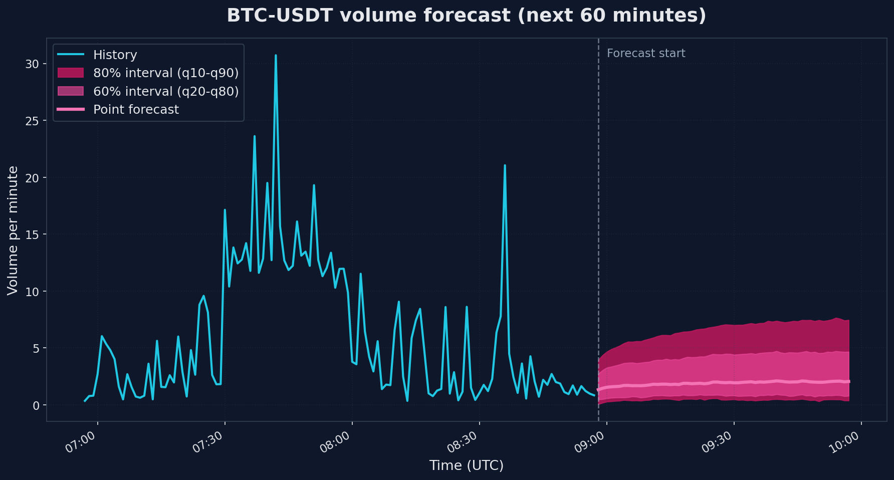
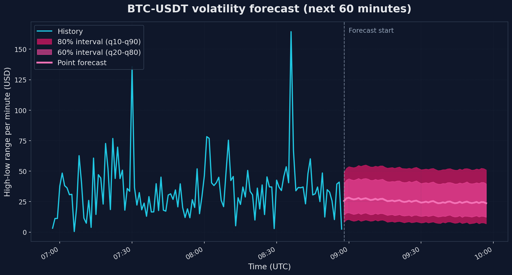
The two charts show very different uncertainty patterns. Volume on the left has a point forecast that drifts upward modestly, but the 80% band is huge - roughly 0.4 to 6.6 when the most recent observed value was 0.83. That is the model saying "I cannot pin this down". Volatility on the right is similar in spread (the 80% band is $8.40 to $52.36) but the point forecast holds fairly steady around $25 because volatility tends to cluster: high-volatility minutes usually follow high-volatility minutes, and the model picks up on that even though it cannot predict which specific minute will spike.
A useful rule of thumb: if the q90/q10 ratio is more than ~3x the point forecast (which it is for volume here), treat the prediction as a directional signal rather than a point estimate. "The next hour looks like normal trading, no liquidity drought, no crisis spike" is genuinely useful information - but do not size your orders on the point number.
Why volume is hard
Volume forecasting on minute bars is genuinely harder than the temperature, electricity, and traffic series TimesFM was trained on. Those have clear diurnal cycles, slow trends, and physical constraints. Trading volume has none of that. It is driven by news, large orders, market microstructure, and herd behavior - all unpredictable from price history alone. The wide intervals are honest, not a model failure.
Limitations and honest assessment
A few important caveats:
- Foundation models are not magic. TimesFM provides a reasonable baseline quickly, but a carefully tuned domain-specific model may perform better for your particular use case.
- This is a data pipeline tutorial. We are showing how to connect QuestDB to TimesFM. Whether the resulting forecasts are useful for your specific application requires proper backtesting and validation.
Conclusion
We covered three methods to move time-series data from QuestDB into a Python ML workflow, each with different trade-offs:
- Direct SQL queries (REST or ConnectorX) - run SQL through QuestDB on every call. Best for exploration and notebooks.
- Parquet export - run SQL once, write the result to a file you can reuse across many training runs. Best for reproducible training pipelines.
- Direct Parquet partition access - bypass the query engine, read the files QuestDB has already materialized. Best for lakehouse-style ML and distributed processing.
We used TimesFM to make this concrete, but TimesFM is one point on a wider spectrum of forecasting approaches:
- Zero-shot foundation models (TimesFM, Chronos, Moirai) - no training required. You get a reasonable baseline immediately. The right starting point when you do not yet know whether the problem is even forecastable.
- Fine-tuned foundation models - same architecture, adapted to your specific data. Better accuracy than zero-shot, much less effort than training from scratch.
- Custom models trained from scratch - LSTMs, Transformers, or classical methods like ARIMA and Prophet. Highest effort, highest ceiling, full control over architecture and features.
The data loading patterns above apply to all three. Whichever approach you end up using, the question of how to get the data out of the database efficiently is the same.
Join our Slack or Discourse communities to share your own forecasting experiments.