Order Book Imbalance Analysis with QuestDB Arrays

Order Book Imbalance Analysis with QuestDB Arrays

Order book imbalance (OBI) is a simple yet powerful metric that measures the disparity between buy and sell orders at different price points in an order book. OBI provides insight into short-term price pressure that often leads to directional moves, making it an early indicator for traders looking to capitalize on market movements.

Storing order book data to compute OBI with traditional relational databases has been challenging as you need to use multiple columns to store bid/ask prices and bid/ask volumes at each price level. A sample schema to capture that market data may look like the following:

CREATE TABLE market_data (
 timestamp TIMESTAMP,
 symbol SYMBOL,
 bid_price_1 DOUBLE, bid_volume_1 DOUBLE,
 bid_price_2 DOUBLE, bid_volume_2 DOUBLE,
 ask_price_1 DOUBLE, ask_volume_1 DOUBLE,
 ask_price_2 DOUBLE, ask_volume_2 DOUBLE,
) TIMESTAMP(timestamp) PARTITION BY HOUR;

Then you would need to aggregate those columns to calculate total liquidity and calculate other metrics for further analysis. With QuestDB 9.0, representing this data has become significantly easier with N-dimensional array types. Instead of storing each price and volume level in separate columns, you can store them in NumPy-like arrays and make use of array functions like array_avg, array_sum, array_count, and array_stddev_samp for simple analysis. In other words, the table schema can be represented cleanly like the following instead:

CREATE TABLE market_data (
  timestamp TIMESTAMP,
  symbol SYMBOL,
  bids DOUBLE[][],
  asks DOUBLE[][]
) TIMESTAMP(timestamp) PARTITION BY HOUR;

In this tutorial, let’s take a look at analyzing order book imbalance using synthetic Bitcoin data. You can follow along by downloading the sample parquet data hosted on GitHub or modify the script to generate your own dataset.

Setting up QuestDB

If you haven’t already done so, download the sample market data parquet file or run the script yourself to generate one. The script will create a synthetic Bitcoin dataset that will create four different scenarios: normal trading conditions, whale accumulation (buy pressure), liquidity crises (sell pressure), and spoofing attempts.

Next, let’s fire up QuestDB and Grafana via Docker Compose so we can explore the data. We’ll also mount the parquet file into the QuestDB container directly, or you can use the QuestDB Python client library to load the dataframe into QuestDB. The Docker Compose yaml file is also available at the sample repository.

From the same folder where you have the docker-compose.yml' file, run docker compose up`.

Now navigate to http://localhost:9000 and we can interact with our parquet file directly from the QuestDB web interface.

For convenience, let’s create a table called market_data with the contents of our parquet file:

CREATE TABLE market_data AS (
SELECT *
FROM read_parquet('btc_order_book_samples.parquet'));

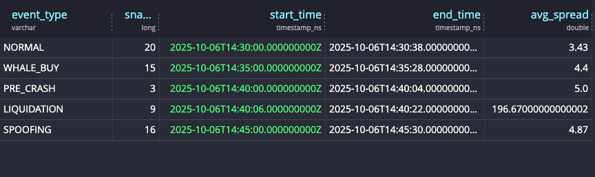
We can run a quick validation query to check what event types we have in the dataset as well as some average spreads for those scenarios:

SELECT
   event_type,
   count() as snapshots,
   min(timestamp) as start_time,
   max(timestamp) as end_time,
   round(avg(asks[1][1] - bids[1][1]), 2) as avg_spread
FROM market_data
GROUP BY event_type
ORDER BY start_time;

Now we’re ready to explore our data!

Exploring order book imbalance

Let’s quickly revisit the definition of order book imbalance. OBI at time t is defined as:

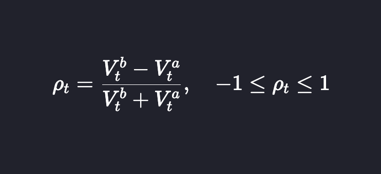
Where Vtᵇ is the bid volume at time t and Vtᵃ is the ask volume at time t. Pₜ between –1 and –⅓ implies sell-heavy, whereas ⅓ to 1 means buy-heavy.

Since OBI looks at the total amount of volume, which may include some old orders, it’s sometimes useful to use the order-flow imbalance metric, which looks at the volume of more recent orders. This can be calculated using level 3 data or changes in the order book.

Normal market conditions

Let’s look at the imbalance metrics under normal market conditions.

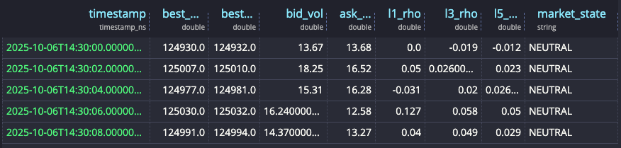
DECLARE
   @thresh := 0.33,
   @state_buy := 'BUY-HEAVY',
   @state_sell := 'SELL-HEAVY',
   @state_neutral := 'NEUTRAL'

WITH base AS (
 SELECT
   timestamp,
   bids,
   asks,
   bids[2] AS bid_vols,
   asks[2] AS ask_vols
 FROM market_data
 WHERE event_type = 'NORMAL'
),
metrics AS (
 SELECT
   timestamp,

   -- top-of-book prices
   round(bids[1][1], 0) AS best_bid,
   round(asks[1][1], 0) AS best_ask,

   -- L1 volumes
   round(bid_vols[1], 2) AS bid_vol,
   round(ask_vols[1], 2) AS ask_vol,

   -- L1 imbalance
   (bid_vols[1] - ask_vols[1])
     / NULLIF(bid_vols[1] + ask_vols[1], 0) AS l1_rho,

   -- Top-3 imbalance (levels 1..3)
   (array_sum(bid_vols[1:4]) - array_sum(ask_vols[1:4]))
     / NULLIF(array_sum(bid_vols[1:4]) + array_sum(ask_vols[1:4]), 0) AS l3_rho,

   -- Top-5 imbalance (levels 1..5)
   (array_sum(bid_vols[1:6]) - array_sum(ask_vols[1:6]))
     / NULLIF(array_sum(bid_vols[1:6]) + array_sum(ask_vols[1:6]), 0) AS l5_rho
 FROM base
)
SELECT
 timestamp,
 best_bid,
 best_ask,
 bid_vol,
 ask_vol,
 round(l1_rho, 3) AS l1_rho,
 round(l3_rho, 3) AS l3_rho,
 round(l5_rho, 3) AS l5_rho,
 CASE
   WHEN l3_rho >  @thresh  THEN @state_buy
   WHEN l3_rho < -@thresh  THEN @state_sell
   ELSE                         @state_neutral
 END AS market_state
FROM metrics
ORDER BY timestamp
LIMIT 5

When we run the query, we can see that under normal market conditions, the imbalance metric stays within –0.1 and 0.1, indicating a balanced order flow.

Market imbalance

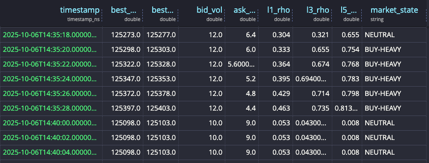
We can update the query above to remove the event_type = 'NORMAL' filter to see how the OBI metric changes in different market states.

You can see the high ρ values in BUY-HEAVY states as well as very negative ρ values for SELL-HEAVY states as built into our dataset with whale-buy and liquidation events.

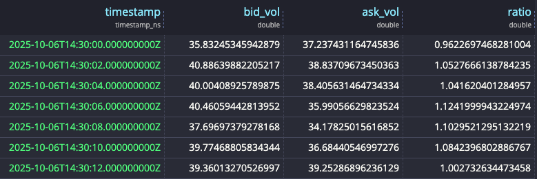
You can also aggregate bid and ask volumes across different levels of the book and quickly see the buy-vs-sell ratio.

DECLARE
 @bid_volumes := bids[2],
 @ask_volumes := asks[2]
SELECT
 timestamp,
 array_sum(@bid_volumes[1:4]) bid_vol,
 array_sum(@ask_volumes[1:4]) ask_vol,
 bid_vol / ask_vol ratio
FROM market_data
ORDER BY timestamp;

Quote spoofing

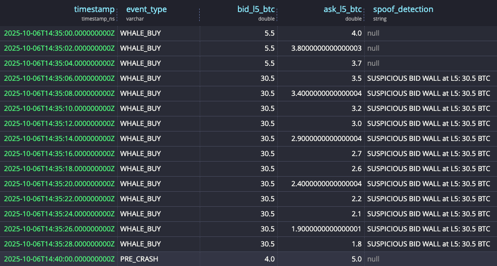
Let’s also detect spoofing attempts where there are large fake walls to create a false impression of depth. In the synthetic data, we put some large fake orders in level 5, so we can directly query for that:

DECLARE
   @bid_volumes := bids[2],
   @ask_volumes := asks[2],

SELECT
   timestamp,
   event_type,
   round(@bid_volumes[5], 1) as bid_l5_btc,
   round(@ask_volumes[5], 1) as ask_l5_btc,
   CASE
       WHEN @bid_volumes[5] > 20 THEN 'SUSPICIOUS BID WALL at L5: ' || round(@bid_volumes[5], 1) || ' BTC'
       WHEN @ask_volumes[5] > 20 THEN 'SUSPICIOUS ASK WALL at L5: ' || round(@ask_volumes[5], 1) || ' BTC'
   END as spoof_detection
FROM market_data
WHERE event_type != 'NORMAL'
ORDER BY timestamp;

And we see them flagged as below.

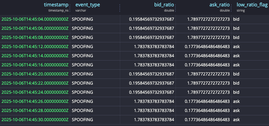
We can also use ratios to detect suspicious bid/ask walls:

SELECT
 timestamp,
 event_type,
 bid_ratio,
 ask_ratio,
 CASE
   WHEN bid_ratio < 0.25 AND ask_ratio < 0.25 THEN 'both'
   WHEN bid_ratio < 0.25 THEN 'bid'
   WHEN ask_ratio < 0.25 THEN 'ask'
 END AS low_ratio_flag
FROM (
 SELECT
   timestamp,
   event_type,
   CASE
     WHEN array_avg(bid_volumes[3:6]) = 0 THEN CAST(NULL AS DOUBLE)
     ELSE array_avg(bid_volumes[1:2]) / array_avg(bid_volumes[3:6])
   END AS bid_ratio,
   CASE
     WHEN array_avg(ask_volumes[3:6]) = 0 THEN CAST(NULL AS DOUBLE)
     ELSE array_avg(ask_volumes[1:2]) / array_avg(ask_volumes[3:6])
   END AS ask_ratio
 FROM (
   SELECT
     timestamp,
     event_type,
     bids[2] AS bid_volumes,
     asks[2] AS ask_volumes
   FROM market_data
 )
)
WHERE bid_ratio < 0.25 OR ask_ratio < 0.25
ORDER BY timestamp;

Visualizing via Grafana

Now let’s visualize the order-book imbalance using Grafana. Navigate to http://localhost:3000 and use the default admin / admin credentials to log in. Under Administration → Plugins and data → Plugin, search for QuestDB and install it.

Then click the blue box to add a new data source. Configure with the following settings:

Server address: questdb
Server port: 8812
Username: user
Password: quest
TLS/SSL mode: disable

We can make a heatmap with OBI distribution. Create a new Dashboards, add a new Panel, and select the Heatmap visualization. If you are using the data from the parquet file, make sure you select the time range '2025-10-06 14:30:00' - '2025-10-06 14:45:00' for UTC on the date picker. If you changed the script, adjust accordingly to the timeframe you ingested, as otherwise you will get an empty panel. You also need to make sure to click on Calculate from data in the right-hand panel.

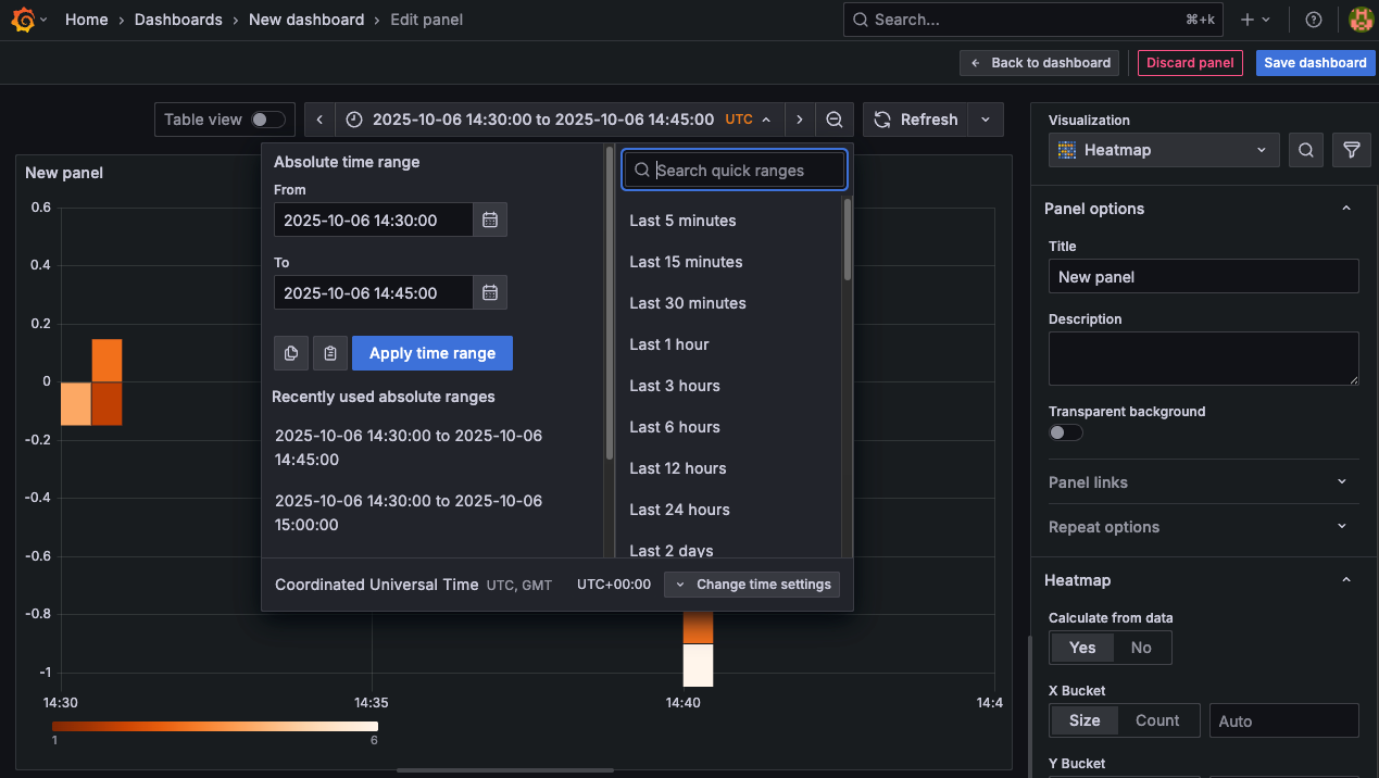
Then in Queries → SQL Editor, paste the following:

WITH base AS (
 SELECT
   timestamp,
   bids,
   asks,
   bids[2] AS bid_vols,
   asks[2] AS ask_vols
 FROM market_data
),
metrics AS (
 SELECT
   timestamp,

   -- top-of-book prices (kept in case you want to use later)
   round(bids[1][1], 0) AS best_bid,
   round(asks[1][1], 0) AS best_ask,

   -- L1 volumes
   round(bid_vols[1], 2) AS bid_vol,
   round(ask_vols[1], 2) AS ask_vol,

   -- L1 imbalance (rho)
   (bid_vols[1] - ask_vols[1]) / NULLIF(bid_vols[1] + ask_vols[1], 0) AS l1_rho
 FROM base
)
SELECT
 timestamp AS "time",
 l1_rho     AS value,
FROM metrics
WHERE $__timeFilter(timestamp) AND l1_rho IS NOT NULL
ORDER BY "time";

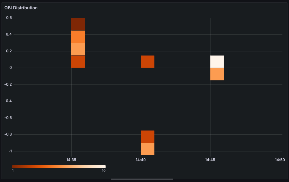
We can zoom in and out on our dataset to see the density of the OBI metric.

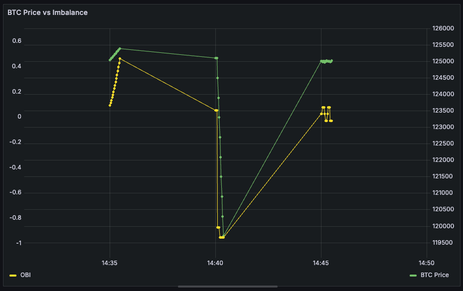
Alternatively, we can plot OBI against BTC price in a timeseries panel. Use a timeseries panel and choose the following query:

SELECT
 timestamp AS time,
 (bids[1][1] + asks[1][1]) / 2 AS "BTC Price",
 (bids[2][1] - asks[2][1]) / NULLIF(bids[2][1] + asks[2][1], 0) AS "OBI"
FROM market_data
WHERE $__timeFilter(timestamp);

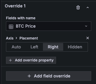
To get dual axes, go to the Overrides panel and put the appropriate settings.

Then we can see a nice graph with both metrics.

Conclusion

In this tutorial, we leveraged QuestDB’s new N-dimensional arrays to run order-book-imbalance analysis with our synthetic Bitcoin data.

Compared to traditional approaches where storing deep levels of orders requires multiple columns, you can now use familiar NumPy-like syntax to run fairly complex analysis with compact 2D array representation.

With array functions built into the database semantics, you don’t have to export your data into a Jupyter notebook to run analysis and build nice visualizations using database features optimized for these workflows.

Even though we used fake data for demonstration, you can obtain a Coinbase or Binance API key to pull level 2 or level 3 data and try this analysis using real order-book data!