Building Real-Time Bollinger Bands Charts with SQL and Grafana
Bollinger Bands are one of the most widely used technical indicators in trading, and for good reason: they turn price volatility into something you can see at a glance. The concept is simple, a moving average with upper and lower bands based on standard deviation. When price touches or breaks through the bands, it's at an extreme relative to recent volatility. That's not a signal on its own, but combined with other indicators, it helps traders spot potential reversals and breakout opportunities.
In this post, I'll show you how to calculate Bollinger Bands using SQL, visualize them in Grafana, and then overlay them on candlestick charts alongside other indicators. This is exactly the approach we use in our live FX order book dashboard.
What are Bollinger Bands?
Bollinger Bands consist of three lines:
- Middle Band: A simple moving average (SMA), typically over 20 periods
- Upper Band: The SMA plus 2 standard deviations
- Lower Band: The SMA minus 2 standard deviations
The bands expand when volatility increases and contract when the market is quiet. When the bands contract tightly (a "squeeze"), it often precedes a significant price move, though the direction must be determined using other indicators. Traders use Bollinger Bands to spot potential breakouts, gauge trend strength, and identify mean reversion opportunities.
Calculating Bollinger Bands in QuestDB
Here's the SQL to calculate Bollinger Bands using 15-minute OHLC candles with a 20-period window. You can run this query on our public demo to see live results.
INFO
The QuestDB demo uses simulated FX data anchored to real reference prices. Volatility may differ from live markets. See the demo data schema for details.
WITH stats AS (SELECTtimestamp,symbol,close,AVG(close) OVER (PARTITION BY symbolORDER BY timestampROWS BETWEEN 19 PRECEDING AND CURRENT ROW) AS sma20,AVG(close * close) OVER (PARTITION BY symbolORDER BY timestampROWS BETWEEN 19 PRECEDING AND CURRENT ROW) AS avg_close_sqFROM market_data_ohlc_15mWHERE timestamp > dateadd('d', -1, now())AND symbol = 'EURUSD')SELECTtimestamp,sma20,sma20 + 2 * sqrt(avg_close_sq - (sma20 * sma20)) AS upper_band,sma20 - 2 * sqrt(avg_close_sq - (sma20 * sma20)) AS lower_bandFROM statsORDER BY timestamp;
Example output
| timestamp | sma20 | upper_band | lower_band |
|---|---|---|---|
| 2026-01-25T14:30:00.000000Z | 1.1793 | 1.1933 | 1.1653 |
| 2026-01-25T14:45:00.000000Z | 1.1796 | 1.1937 | 1.1655 |
| 2026-01-25T15:00:00.000000Z | 1.1791 | 1.1935 | 1.1648 |
| 2026-01-25T15:15:00.000000Z | 1.1785 | 1.1914 | 1.1656 |
| 2026-01-25T15:30:00.000000Z | 1.1788 | 1.1913 | 1.1663 |
| 2026-01-25T15:45:00.000000Z | 1.1781 | 1.1907 | 1.1655 |
| 2026-01-25T16:00:00.000000Z | 1.1778 | 1.1903 | 1.1653 |
Notice how the bands contract as volatility decreases: at 14:30 the band width is about 280 pips, narrowing to 250 pips by 16:00. Traders watch for this contraction (a "squeeze") as it often precedes significant price moves. You can quantify this with Bollinger BandWidth, which expresses the width as a percentage and compares it to historical levels, making it easier to spot when volatility is near its 6-month lows.
The query uses the variance formula sqrt(avg(x²) - avg(x)²) to calculate standard deviation. This uses population standard deviation rather than sample standard deviation, which is common in trading platforms.
With 20 periods of 15-minute candles, the SMA covers a 5-hour window. You can adjust the period count and candle size to match your trading timeframe.
For more variations and detailed explanations, see our Bollinger Bands cookbook recipe.
Visualizing Bollinger Bands in Grafana
Running the query above in Grafana gives you a clean visualization of the three bands:
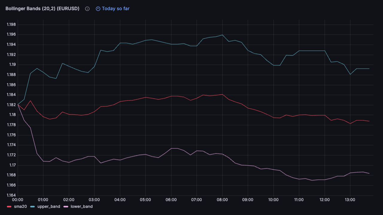
This is useful for seeing volatility patterns, but in practice you want to see the bands in context with actual price movement.
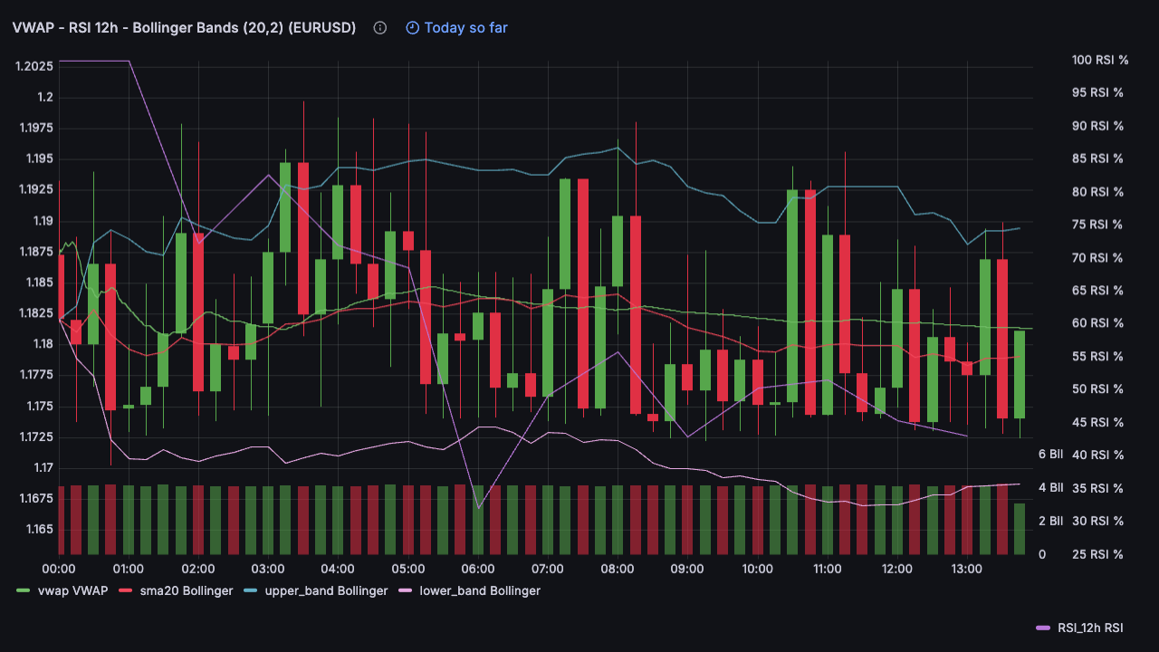
Overlaying Indicators on Candlestick Charts
The real power comes from overlaying Bollinger Bands on top of OHLC candlesticks, alongside other indicators like VWAP or RSI. This gives you a complete picture of price action, volatility, and momentum in a single chart.
The Grafana technique
To build this multi-indicator chart in Grafana:
-
Use the Candlestick visualization as your base chart type
-
Add multiple queries to the same panel: one for OHLC data (your candles), and additional queries for each indicator (Bollinger Bands, VWAP, RSI, etc.)
-
Enable "Include all fields" in the candlestick chart options under "Additional fields". This tells Grafana to render data from all your queries, not just the OHLC fields.
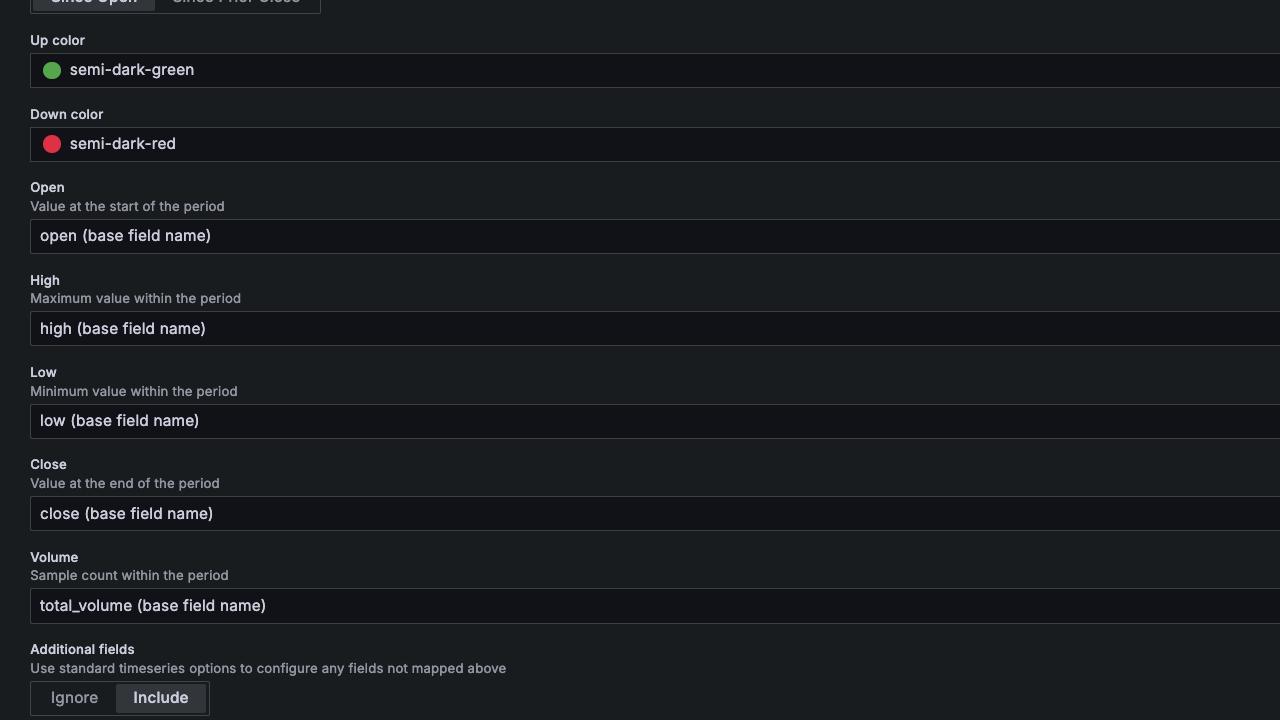
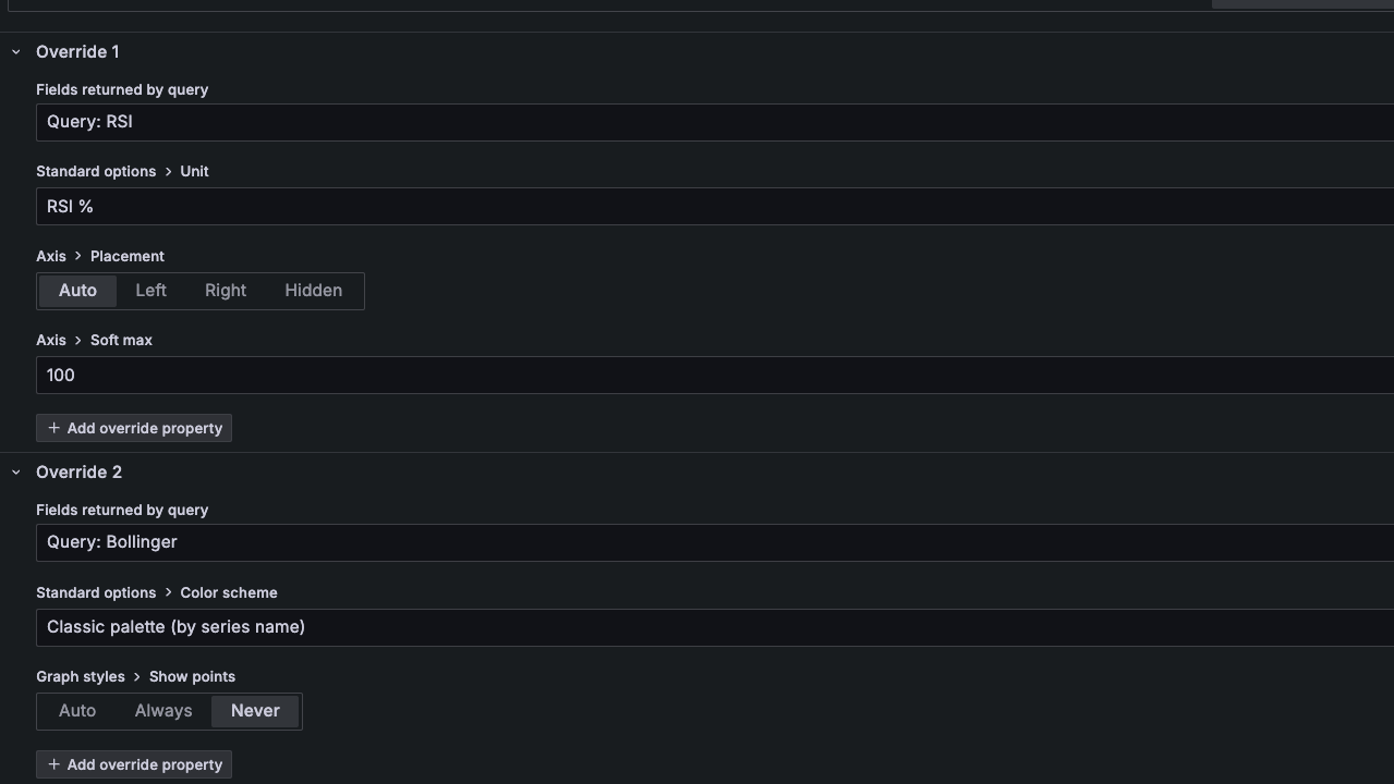
- Use Overrides for styling: Each indicator needs different visual treatment. Use Grafana's override system to set colors, line styles, and axis configuration per query. For example, RSI operates on a 0-100 scale, so you'll want to configure it with a custom unit and place it on the right axis to avoid distorting your price scale.
This same technique works for any combination of indicators. In the example above, I'm showing VWAP (volume-weighted average price) and a 12-hour RSI alongside the Bollinger Bands, each with their own color scheme and axis configuration.
See it live
You can explore this visualization with real-time FX data on our live FX order book dashboard. The chart in the second row shows Bollinger Bands overlaid on 15-minute candles, defaulting to EUR/USD with other major currency pairs available via the symbol selector.
For the complete SQL and more examples, check out the Bollinger Bands cookbook recipe.