How to Build Market Depth Charts from Order Book Data with QuestDB
If you've ever looked at a trading terminal or watched market data flow by, you've probably noticed those waterfall-like charts showing layers of buy and sell orders stacked at different price levels. These are market depth charts, and they're one of the most valuable tools for understanding what's really happening in a market at any given moment.
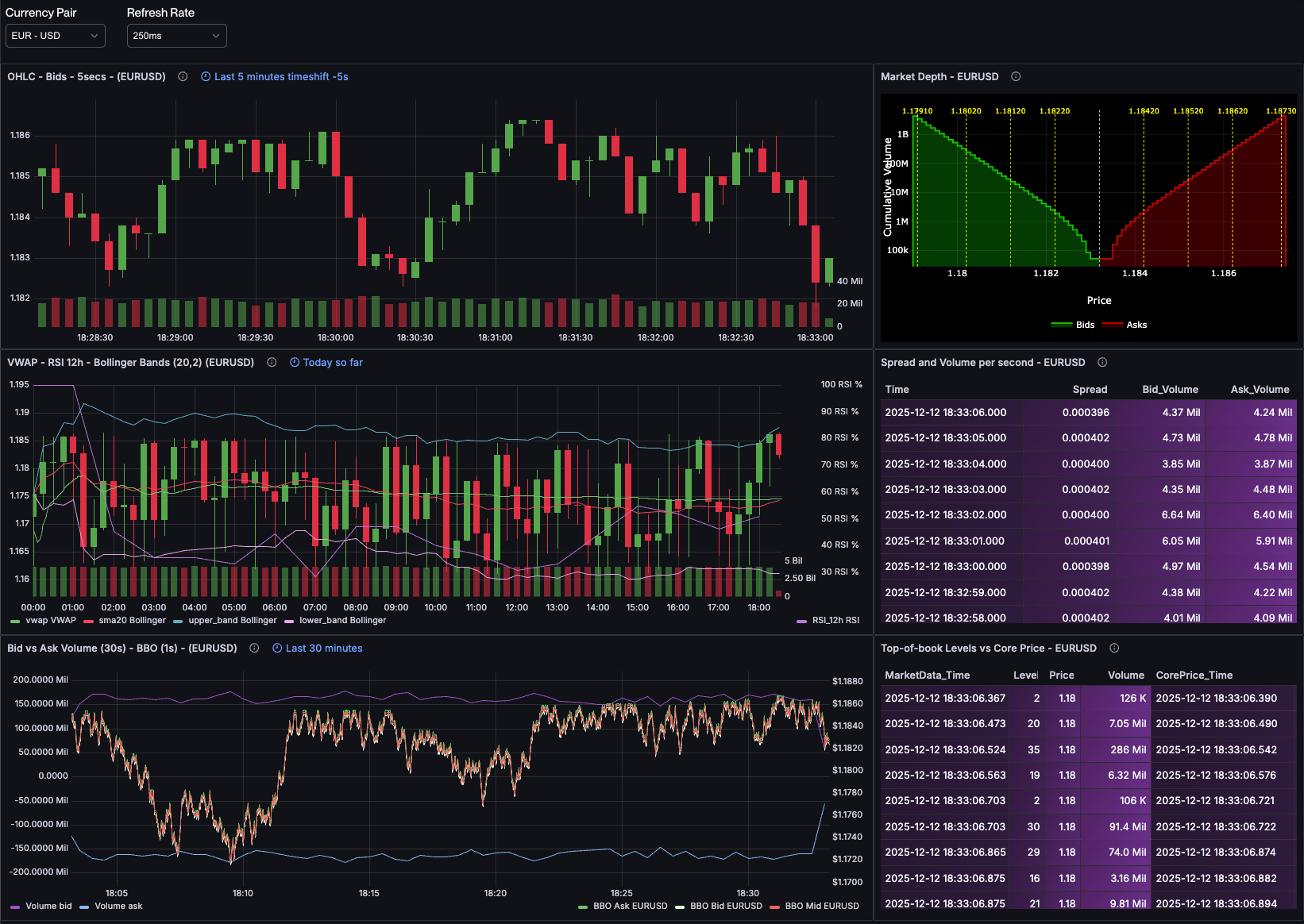
In this post, I'll walk through how to store order book data efficiently in QuestDB using arrays, and then show you how to transform that data into market depth visualizations using SQL. By the end, you'll understand not just how to build these charts, but why they matter for anyone working with financial data. In fact, the techniques we'll cover here are exactly what power the market depth chart (top right panel) in our live FX order book dashboard, which visualizes real-time EUR/USD, GBP/USD, and other major currency pairs.
Understanding Order Books and Market Depth Charts
Before we dive into the technical implementation, let's talk about what we're actually modeling here. If you're already familiar with order books and market making, feel free to skip ahead. But if terms like "best bid" and "order book levels" sound like financial jargon, stick with me for a moment.
The Order Book: A Market's Memory
An order book is essentially a live snapshot of supply and demand for a financial instrument. Think of it as a two-sided auction that never stops. On one side, you have buyers (the "bid" side) saying "I want to buy at this price." On the other side, you have sellers (the "ask" or "offer" side) saying "I'll sell at this price."
Each side of the book is organized by price levels. A price level is simply a price point where one or more orders are waiting. For example, if three different traders want to buy EUR/USD at 1.1650, that becomes one price level with the combined volume from all three orders.
Here's where it gets interesting: the bid side is sorted in descending order by price (highest bids first), while the ask side is sorted in ascending order (lowest asks first). This makes intuitive sense: buyers want to pay as little as possible, but the highest bidders get priority. Sellers want to receive as much as possible, but the lowest asking prices get matched first.
The very best prices on each side are special:
- Best bid: The highest price anyone is willing to pay right now
- Best ask: The lowest price anyone is willing to sell for right now
The difference between these two is the bid-ask spread, and it's one of the most important indicators of market liquidity.
Market Makers and the Shape of Liquidity
Market makers continuously quote both buy and sell prices, providing liquidity so that other traders can execute immediately without waiting for a counterparty. They make money on the spread and the sheer volume of trades, but they take on significant risk in the process.
When a market maker sets their prices, they don't just throw out random numbers. They typically place orders at multiple levels away from the current price, creating a distribution of liquidity. You might see a market maker offering to buy 100,000 EUR at 1.1650, another 100,000 EUR at 1.1645, another 150,000 EUR at 1.1640, and so on. This creates depth in the market.
And here's a key economic principle at play: the worse the price, the more volume you'll typically see. Why? Because traders placing limit orders further from the market price know they're less likely to get filled, so they're willing to commit larger amounts. Conversely, orders very close to the current price are more likely to execute, so traders might be more conservative with size.
This dynamic creates the characteristic "depth curve" that we visualize in market depth charts.
Why Market Depth Charts Matter
A market depth chart shows you the cumulative volume available at each price level. Instead of seeing individual orders, you see the total amount of buying or selling pressure building up as you move away from the current price.
Why is this useful?
-
Liquidity assessment: You can instantly see how much volume would be needed to move the price significantly. A thin market with little depth can be moved with small orders. A deep market with substantial volume at multiple levels is much harder to manipulate.
-
Support and resistance levels: Large concentrations of orders at specific price levels can act as support (on the bid side) or resistance (on the ask side). These are price points where the market is likely to stall or reverse.
-
Market maker behavior: You can see how sophisticated traders are positioning themselves. Are they pulling back liquidity? Are they adding depth at certain levels? This gives you insight into market sentiment.
-
Execution cost estimation: If you need to execute a large order, the depth chart tells you exactly what it will cost. You can see where your order will walk through the book and what your average fill price will be.
Here's an example from one of my dashboards showing EUR/USD market depth:
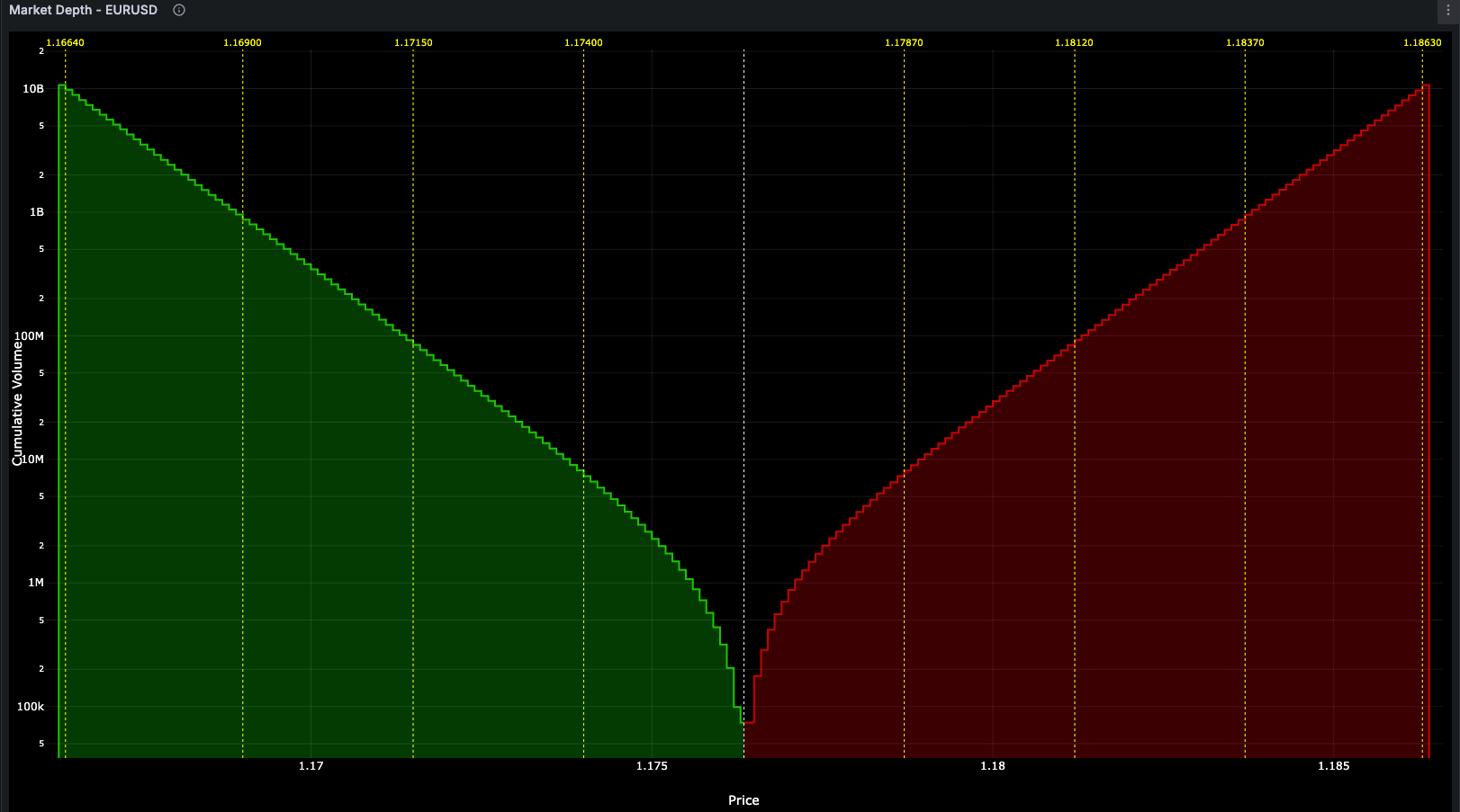
On the left, you see cumulative bid volume building up as prices decrease. On the right, cumulative ask volume increases as prices rise. The gap in the middle is the spread, the no-man's land between buyers and sellers. The vertical lines indicate price barriers where significant volume concentrations exist.
Storing Order Books in QuestDB
Now that we understand what we're modeling, let's talk about how to store this data efficiently. Order books are inherently structured as levels, and in QuestDB, arrays are a perfect fit for this structure.
The Array Approach
Rather than storing each price level as a separate row (which would explode your row count and create performance issues), you can store an entire side of the order book as 2D arrays within a single row. Here's my table schema:
CREATE TABLE market_data (timestamp TIMESTAMP_NS,symbol SYMBOL,bids DOUBLE[][],asks DOUBLE[][]) TIMESTAMP(timestamp) PARTITION BY DAY;
The SYMBOL type is particularly efficient for the currency pair identifier since it uses an
internal dictionary to map strings to integers, reducing storage overhead for this frequently repeated value.
The key insight here is using 2D arrays where the first dimension contains an array of prices and the second contains
an array of volumes, keeping related data naturally paired together. Using TIMESTAMP_NS
gives us nanosecond precision, which is essential for high-frequency market data.
Each snapshot of the order book becomes one row. For example, here's a recent snapshot from my EUR/USD feed:
| timestamp | symbol | bids | asks |
|---|---|---|---|
| 2025-12-12T15:43:17.554207013Z | EURUSD | [[1.1655, 1.1654, 1.1653, ...], [77697.0, 100509.0, 116928.0, ...]] | [[1.1659, 1.1660, 1.1661, ...], [85431.0, 95220.0, 110847.0, ...]] |
The bids[1] array contains bid prices in descending order, and bids[2] contains the corresponding volumes. Similarly,
asks[1] contains ask prices in ascending order, and asks[2] contains volumes.
This compact representation has several advantages:
- Temporal coherence: All price levels from a single snapshot stay together, making it easy to query historical market states
- Efficient storage: 2D array storage is much more space-efficient than separate rows or even separate arrays
- Fast retrieval: Fetching a complete order book snapshot is a single row read
- Natural pairing: Prices and volumes stay naturally aligned through array indexing
Computing Market Depth Charts with SQL
Here's where QuestDB's SQL array functions really shine. To create a market depth
chart, we need to compute cumulative
sums of the volumes at each price level. Fortunately, QuestDB has a built-in array_cum_sum()
function that makes this remarkably simple.
Cumulative Sum Query
Here's the query I use to compute cumulative depth for the most recent order book snapshot:
WITH snapshot AS (SELECT timestamp, bids, asksFROM market_dataWHERE symbol = 'EURUSD'LATEST ON timestamp PARTITION BY SYMBOL)SELECTtimestamp,bids[1] as bprices,bids[2] as bvolumes,array_cum_sum(bids[2]) as bcumvolumes,asks[1] as aprices,asks[2] as avolumes,array_cum_sum(asks[2]) as acumvolumesFROM snapshot;
Let's break down what's happening:
- snapshot CTE: Fetches the most recent order book snapshot for EUR/USD using
LATEST ON. - Array extraction:
bids[1]extracts the price array,bids[2]extracts the volume array - Cumulative sum:
array_cum_sum(bids[2])computes the running total of bid volumes across all price levels - Same for asks: We do the same extraction and cumulative sum for the ask side
The beauty of this approach is how concise it is. The array_cum_sum() function handles all the complexity of iterating
through the array and computing running totals.
Example Output
Here's actual output from my EUR/USD feed (showing abbreviated arrays for readability):
| timestamp | bprices | bvolumes | bcumvolumes | aprices | avolumes | acumvolumes |
|---|---|---|---|---|---|---|
| 2025-12-12T15:43:23.664356301Z | [1.1647, 1.1646, 1.1645, 1.1644, ...] | [77697.0, 100509.0, 116928.0, 128535.0, ...] | [77697.0, 178206.0, 295134.0, 423669.0, ...] | [1.1651, 1.1652, 1.1653, 1.1654, ...] | [85431.0, 95220.0, 110847.0, 125340.0, ...] | [85431.0, 180651.0, 291498.0, 416838.0, ...] |
The result returns arrays for everything:
- bprices/aprices: The actual price levels on each side
- bvolumes/avolumes: The volume available at each price level
- bcumvolumes/acumvolumes: The cumulative volume (running total)
For visualization, you typically zip these arrays together (prices with cumulative volumes) to plot the depth curve. At price level 1.1644 on the bid side, there's a cumulative 423,669 units of EUR available for purchase. On the ask side at 1.1654, there's 416,838 units available for sale.
Visualizing with Grafana and the Plotly plugin
Once you have the query returning cumulative depth data, you need to visualize it. Grafana doesn't have a built-in chart type that's ideal for market depth visualization, so I use a custom visualization built with Plotly.
The basic approach is straightforward:
- Query QuestDB with the market depth SQL shown above
- Parse the returned arrays (bprices, bcumvolumes, aprices, acumvolumes)
- Create two line traces in Plotly: one for bid depth, one for ask depth
- Plot price on the x-axis and cumulative volume on the y-axis
- Add vertical lines to indicate price barriers where significant volume concentrations exist
I refresh this visualization every 250ms to keep it real-time. At that frequency, you can actually watch the order book breathe, seeing liquidity appear and disappear as market makers adjust their quotes and traders place or cancel orders.
The key is that the SQL query is fast enough (typically about 300 microseconds) that even at 250ms refresh intervals, there's minimal overhead. QuestDB's columnar storage and array operations make this kind of high-frequency querying practical.
Extending the Analysis
Market Depth is just one of the tools for order book analytics. Using QuestDB arrays you can easily calculate the bid-ask spread, analyze liquidity to plan executions or for backtesting, find the order book imbalance, detect volume dropoffs... all of them with the best possible performance. Check out our post about Order Book analytics for more information.
Wrapping Up
Market depth visualization might seem like a niche use case, but it's a powerful example of how array types in time-series databases can elegantly solve real-world problems. By storing order book levels as 2D arrays in QuestDB, we get:
- Compact, efficient storage for complex market data structures
- Fast queries for cumulative depth calculations using
array_cum_sum() - Temporal analysis capabilities to track market microstructure changes
- Sub-10ms query performance enabling 250ms refresh rates for real-time dashboards
If you're working with market data or building trading infrastructure, I'd encourage you to experiment with these array-based patterns. The combination of QuestDB's array operations and nanosecond timestamps makes it particularly well-suited for high-frequency financial data.