Building K-line (Candlestick) Charts with QuestDB and Grafana

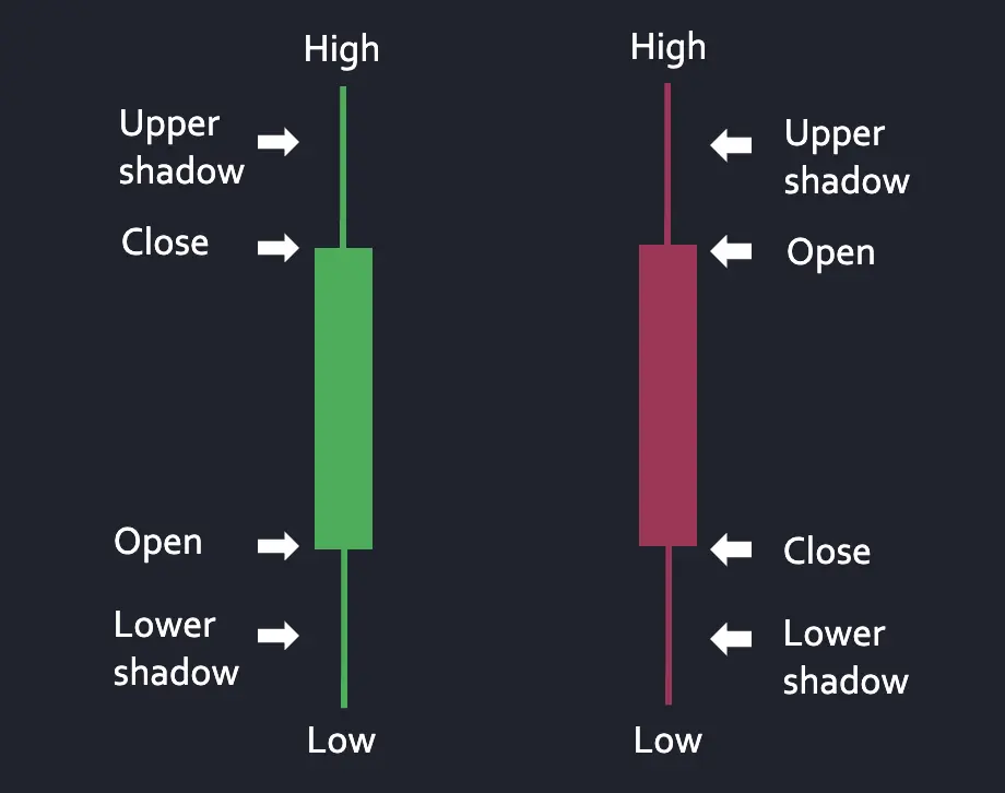
K-line or candlestick charts are a popular way to visualize tick data to show price movement of an asset over time. For a given time window, each k-line chart shows the open, high, low, and close (OHLC) data points as well as the price movement via color (green for positive, where close price is higher than open price, and red for negative).

In this tutorial, we will stream real-time crypto data from polygon.io and utilize QuestDB’s new materialized view functionality to create aggregated OHLC tables efficiently. We will then visualize them via k-line charts in Grafana.

Setting up QuestDB and Grafana

Before getting started with our data ingestion, let’s startup QuestDB and Grafana via Docker Compose. For this exercise, we will utilize the Postgres Wire port (8812) to both ingest data and for Grafana to connect to pull data. Since the materialized view feature is still in beta, we need to set QDB_CAIRO_MAT_VIEW_ENABLED to true prior to starting up QuestDB.

Create docker-compose.yml file as below:

version: '3.8'

services:
 questdb:
   image: questdb/questdb:latest
   container_name: questdb
   ports:
     - "8812:8812"
     - "9000:9000"
   environment:
     - QDB_CAIRO_MAT_VIEW_ENABLED=true
     - QDB_PG_READONLY_USER_ENABLED=true

 grafana:
   image: grafana/grafana:latest
   container_name: grafana
   ports:
     - "3000:3000"
   depends_on:
     - questdb

Then run it in the background via: docker compose up -d. Navigate to localhost:9000 (QuestDB’s UI) and localhost:3000 (Grafana’s UI) to make sure both are running.

Streaming Crypto Data via Polygon.io

Now that we have QuestDB and Grafana up and running, let’s work on ingesting trades data into QuestDB.

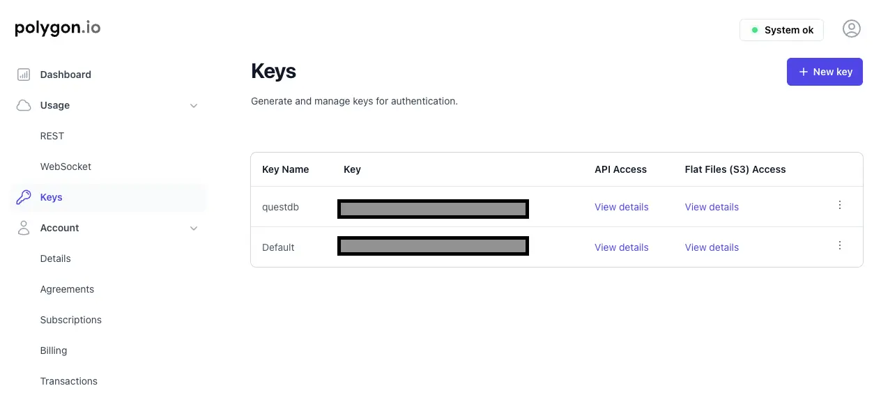
Since Polygon.io provides a nice WebSocket connection to stream real-time trades data from various exchanges, we will use it to populate our raw trades table in QuestDB. The WebSocket feature is part of the “Currencies Starter” package (costs $49/mo), so sign up for the updated account and grab the API key from the dashboard.

Note: if you would rather use a free alternative or ingest data from an exchange not yet supported by Polygon.io, you can follow Ingesting Financial Tick Data Using a Time-Series Database guide.

Next, create requirements.txt and populate with the following:

requirements.txt
websockets
psycopg2
asyncio

Let’s install the required dependencies: pip install -r requirements.txt

Next, let’s create a simple ingest.py file to connect to Polygon.io, subscribe to the crypto WebSocket connection, and stream that into the trades table in QuestDB.

ingest.py
import asyncio
import websockets
import json
import psycopg2
from datetime import datetime, timezone

API_KEY = "<my-api-key-here>"
TICKER = "X:BTC-USD"
QUESTDB_CONN = "host=localhost port=8812 user=admin password=quest"

EXCHANGE_MAP = {
   1: "Coinbase",
   2: "Bitfinex",
   6: "Bitstamp",
   10: "Binance",
   23: "Kraken"
}

def create_trades_table():
   conn = psycopg2.connect(QUESTDB_CONN)
   cursor = conn.cursor()
   cursor.execute("""
       CREATE TABLE IF NOT EXISTS trades (
           timestamp TIMESTAMP,
           ticker SYMBOL,
           price DOUBLE,
           size DOUBLE,
           exchange SYMBOL
       ) TIMESTAMP(timestamp) PARTITION BY DAY;
   """)
   conn.commit()
   cursor.close()
   conn.close()

async def stream_crypto_trades():
   uri = "wss://socket.polygon.io/crypto"
   async with websockets.connect(uri) as ws:
       await ws.send(json.dumps({"action": "auth", "params": API_KEY}))
       await ws.send(json.dumps({"action": "subscribe", "params": f"XT.{TICKER}"}))

       conn = psycopg2.connect(QUESTDB_CONN)
       cursor = conn.cursor()

       async for message in ws:
           data = json.loads(message)
           for trade in data:
               if trade['ev'] == 'XT':
                   ts = datetime.fromtimestamp(trade['t'] / 1000.0, tz=timezone.utc).strftime('%Y-%m-%dT%H:%M:%S.%fZ')
                   size = float(trade['s']) if isinstance(trade['s'], (float, int)) else 0.0
                   exch = EXCHANGE_MAP.get(trade['x'], f"EX_{trade['x']}")
                   cursor.execute("""
                       INSERT INTO trades (timestamp, ticker, price, size, exchange)
                       VALUES (%s, %s, %s, %s, %s)
                   """, (ts, trade['pair'], trade['p'], size, exch))
                   conn.commit()

if __name__ == "__main__":
   create_trades_table()
   asyncio.run(stream_crypto_trades())

A few things to note here:

• The timestamp field from Polygon.io is in Unix MS so we need to convert it to the correct precision in QuestDB.
• I’m collecting mapping exchange data in the ingestion process, but we can also just join that table in QuestDB. The full list of exchange data is listed here: https://polygon.io/docs/rest/crypto/market-operations/exchanges
• Polygon.io does provide an open to grab custom OHLC bars via its REST API, but we’re electing to build this aggregation ourselves in QuestDB for flexibility and performance reasons.

Run this script to start ingesting data:

python ingest.py

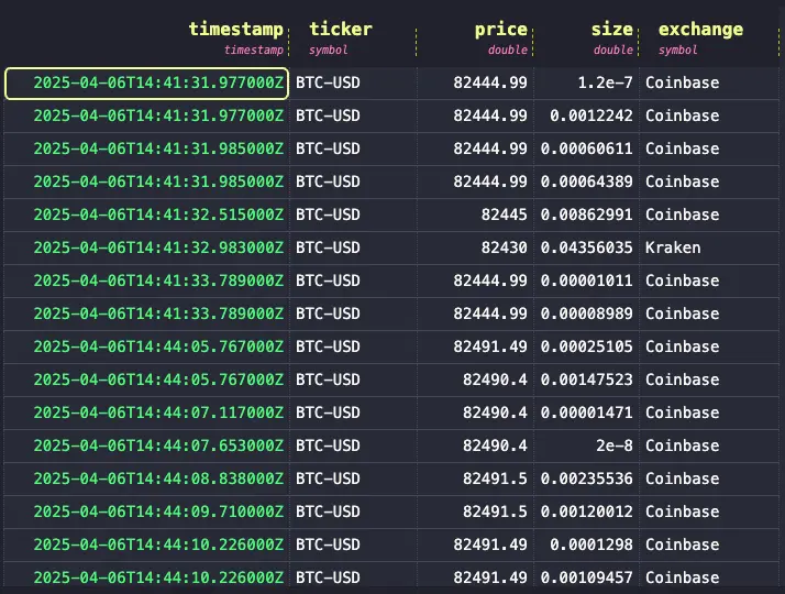
We can validate that data is making it to QuestDB by navigating to the UI and running a simply query like SELECT * FROM trades:

Aggregating trades data via materialized view

With QuestDB 8.2.3, we now have materialized views in beta. Since materialized views persist data to disk instead of computing them at query time like regular views, they are a great fit for creating OHLC aggregation tables that are built on top of our raw trades table. Materialized views also provide an incremental refresh mechanism, which makes the query execution efficient. This way we can avoid having to run expensive aggregate queries frequently (e.g., when creating graphs on Grafana) and instead rely on precomputed values that materialized views provide.

Let’s create some OHLC tables grouped by 1s, 5s, and 1m intervals. Notice that each of these materialized views are chained (i.e., the 5s view is built on top of 1s view), otherwise known as cascaded materialized views.

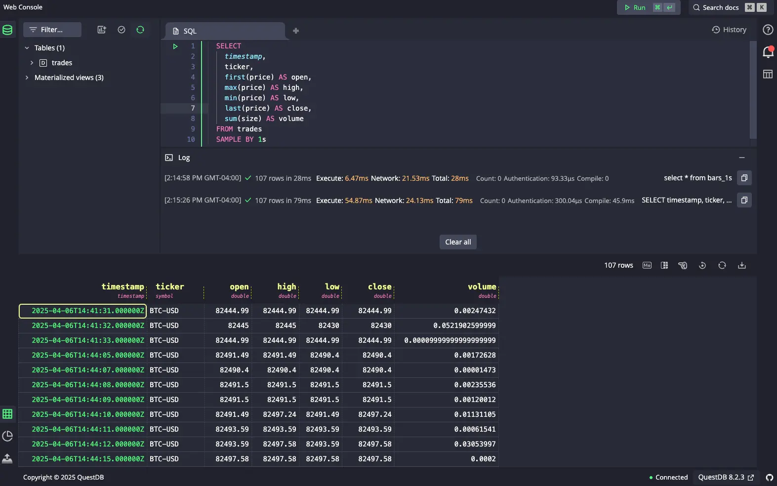
CREATE MATERIALIZED VIEW bars_1s AS (
 SELECT
   timestamp,
   ticker,
   first(price) AS open,
   max(price) AS high,
   min(price) AS low,
   last(price) AS close,
   sum(size) AS volume
 FROM trades
 SAMPLE BY 1s
) PARTITION BY HOUR TTL 1 DAY;

CREATE MATERIALIZED VIEW bars_5s AS (
 SELECT
   timestamp,
   ticker,
   first(open) AS open,
   max(high) AS high,
   min(low) AS low,
   last(close) AS close,
   sum(volume) AS volume
 FROM bars_1s
 SAMPLE BY 5s
) PARTITION BY HOUR BY HOUR TTL 1 DAY;

CREATE MATERIALIZED VIEW bars_1m AS (
 SELECT
   timestamp,
   ticker,
   first(open) AS open,
   max(high) AS high,
   min(low) AS low,
   last(close) AS close,
   sum(volume) AS volume
 FROM bars_5s
 SAMPLE BY 1m
) PARTITION BY HOUR;

Now we can query data against these materialized views:

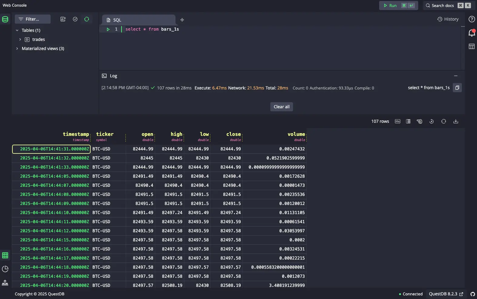
Notice the execution time: 6.47ms. Now if we were to query that exact same data are query time, it would be significantly slower at 54.87ms:

Now we can query data against these materialized views:

The difference in performance would obviously vary depending on the size of the data, and how many clients are hitting this endpoint. But you can imagine that at scale, utilizing a materialized view would be a significant performance boost than using regular views or periodically updating tables.

Visualizing via Grafana

Finally, let’s construct our k-line graph on Grafana. Navigate to localhost:3000 and login as the default admin user (username: admin, password: admin). Then under Data Sources, search for QuestDB datasource. Since we’re running in Docker and we named the QuestDB component as questdb, enter questdb for the server address and 8812 for our Postgres wire port. We will also use our read-only user (username: user, password: quest). Make sure to disable TLS / SSL settings and click “Save & test”.

Grafana comes with a built-in Candlestick plugin, so we can start creating our dashboard. Click on Dashboards to open “Add visualization”. Select our QuestDB datasource, and under the SQL Editor, we can select our query. We can just select our fields from bars_5s table for example:

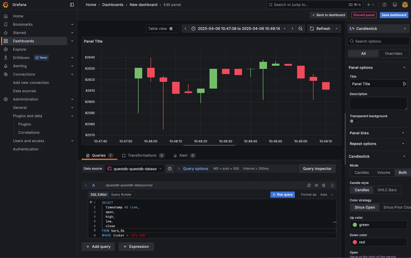
SELECT
 timestamp AS time,
 open,
 high,
 low,
 close
FROM bars_5s
WHERE ticker = 'BTC-USD'
ORDER BY timestamp

Then on the right hand side, change the Time series option to Candlestick and the default options will create our k-line / candlestick chart.

Wrapping up

In this tutorial, we looked at creating a k-line chart by pulling real time trades data from Polygon.io and using materialized views to efficiently aggregate OHLC data on QuestDB. We can extend this demo to ingest not only BTC-USD pairs but also other cryptocurrencies. Since we are collecting exchange information as well, we can create materialized views that split out not only asset pairs but also by exchange as well.

One more thing to note: in this tutorial, we used the PGwire to insert data. At low-volume, the PGwire protocol is a convenient way to insert data into QuestDB. However, high throughput is expected or if insert performance is paramount, then utilizing the Influx Line Protocol (ILP) is the better option. You can follow “Analyzing Bitcoin Options Data with QuestDB” for an example of utilizing ILP.