Exploring high resolution foreign exchange (FX) data

In a previous post, we looked at FX rates from the European Central Bank (ECB) over a period of multiple years. Looking at these rates was a useful way to explore some important parts of European history through a financial lens. While extensive, this dataset was relatively sparse as it only included daily fixings for the currency pairs in scope.

In this post, we'll increase the resolution and look at intraday FX data using some of QuestDB's oldest and newest finance functions. High-frequency FX data provides a granular view of market movements, capturing every tick and allowing for detailed analysis of trading patterns and market behavior.

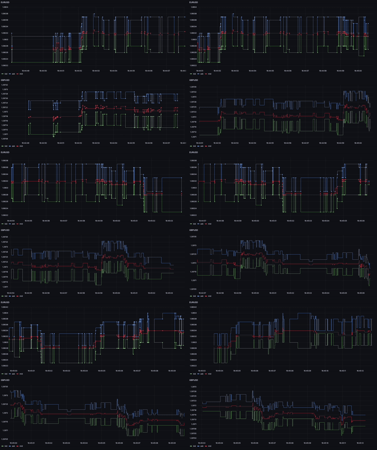
Before we dive in, here's a realtime replay to give a sense of the dataset resolution. The width of the chart window is 10 seconds:

About the dataset

Getting our hands on high-resolution quality market data can be challenging. Some platforms, such as crypto exchanges, offer it for free via an API, while other data is often behind a paywall. In this instance, TrueFx offers historical CSV downloads on their website after creating an account. This is a nice opportunity to play with high-resolution FX data.

As currencies trade over the counter, there is no centralized exchange reporting market data. Instead, the dataset is composed of contributions from FX dealing banks, brokers, and asset managers. What's nice about this dataset is that it provides tick-by-tick prices, with a resolution up to a millisecond.

High-resolution data is valuable because it allows traders and analysts to observe market dynamics in real-time, identify trends, and make informed decisions based on the most current information.

The CSV files look like the following:

~/D/october> head EURUSD-2024-10.csv 
EUR/USD,20241009 14:40:21.818,1.09476,1.09478
EUR/USD,20241009 14:40:21.912,1.09473,1.09482
EUR/USD,20241009 14:40:22.131,1.09476,1.09478
EUR/USD,20241009 14:40:22.600,1.09473,1.09482
EUR/USD,20241009 14:40:22.615,1.09471,1.09483
EUR/USD,20241009 14:40:22.631,1.09476,1.09478
EUR/USD,20241009 14:40:22.725,1.09471,1.09484
EUR/USD,20241009 14:40:22.740,1.09472,1.09482

Ingesting the dataset

After creating an account with TrueFX, we can browse the available files, tick the pairs and intervals we want, and trigger a download. For our cases, each file covers a month.

We import all the files using the Web Console's CSV upload functionality, which creates tables based on the filename such as "USDTRY-2024-10.csv".

Since the files don't contain headers, QuestDB needs to be supplied with a schema. However, it is also possible to import as-is. In this case, the columns would be named f0, f1, etc.

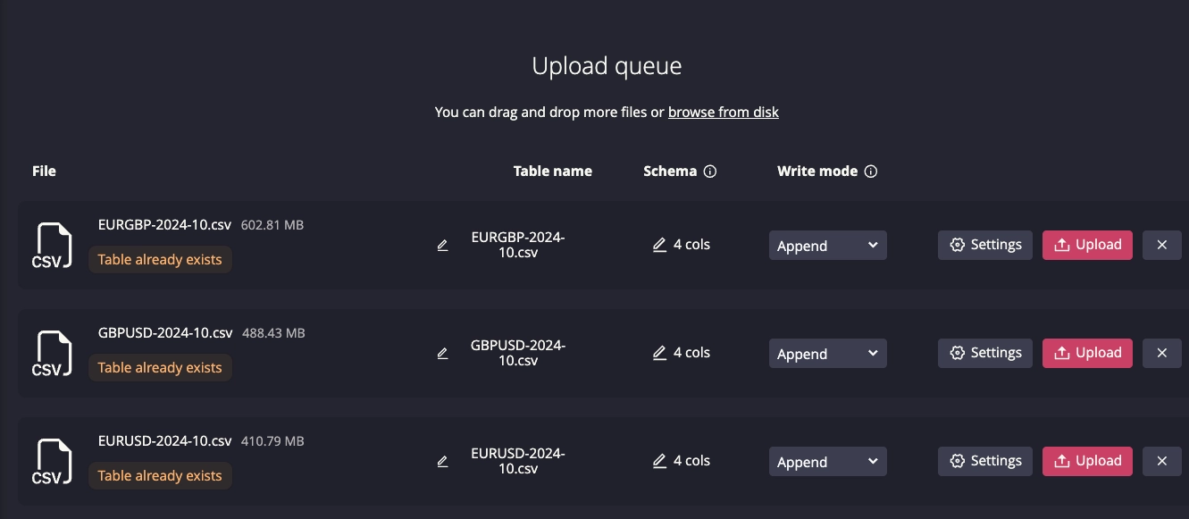
To facilitate downstream analysis, we will join the different files together into one table. To do this, we'll use CREATE TABLE AS coupled with UNION ALL to combine the different CSVs.

We'll also apply ORDER BY timestamp and nominate a designated timestamp column.

Lastly, we'll parse the timestamp as it is displayed with a particular format using the to_timestamp function.

The final query looks like the following:

CREATE TABLE fxrates AS (
    SELECT f0 pair, to_timestamp(f1, 'yyyyMMdd HH:mm:ss.SSS') timestamp, f2 bid, f3 ask
    FROM
    ("EURGBP-2024-10.csv" UNION ALL "EURUSD-2024-10.csv" UNION ALL "GBPUSD-2024-10.csv")
    ORDER BY timestamp asc
) timestamp(timestamp)

Mid price smoothing

The mid function is relatively simple as it's just (bid + ask)/2. Its function is to act as syntactic sugar whenever dealing with price data that shows both sides of the order book.

This way, we can summarize both prices into a single series. Mid-price smoothing is useful because it provides a more stable view of price movements, reducing noise and allowing for clearer trend analysis.

Deriving the mid is as simple as running the following query:

SELECT timestamp, mid(bid,ask) 
FROM fxrates where pair = 'EUR/USD' AND $__timeFilter(timestamp)

The result is the smoother red line which is rendered alongside bid and ask prices on the below chart. The time interval below is only 20 seconds which gives an idea of how frequently the data is updating:

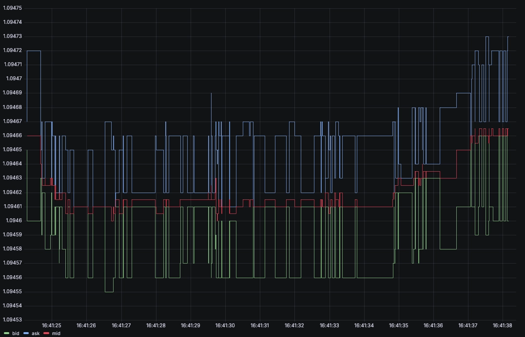
Another nice feature of deriving the mid price is the smoothing effect. At higher resolution, you may often see the top of the book widen on either one side, or both. What can happen, for example, is that someone trades against the dealer on one side, and then they widen their quotes immediately before tightening again.

We can see this effect in the above chart whereby the order book tightenings and widenings seem to always happen in symmetry, which indicates the changes in spread are likely one dealer adjusting their quotes.

We can use a combination of WITH and LT JOIN to join tables based on timestamp. However, LT JOIN performs on timestamp inequality which means that for a given timestamp in the first table, it will join on the first timestamp which is inferior or equal in the second table.

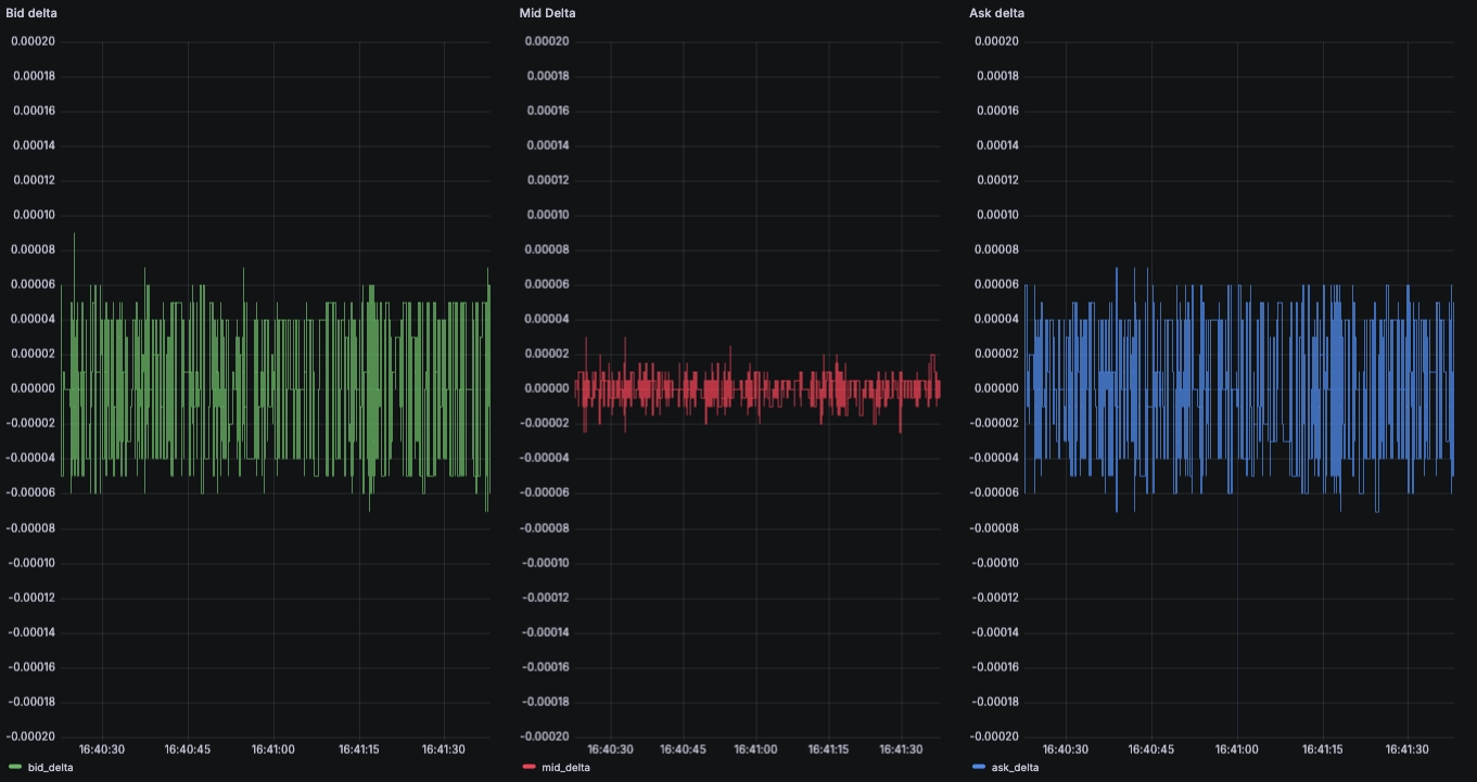
In practice, we can apply LT JOIN on a single table to join it to itself, and this will return both the current value for the timestamp in question, and the immediately preceding value. We can then apply a function to derive values such as the change since the last event:

WITH
a AS (SELECT timestamp, bid FROM fxrates WHERE pair = 'EUR/USD'),
b AS (SELECT timestamp, bid FROM fxrates WHERE pair = 'EUR/USD')
SELECT a.timestamp, b.bid - a.bid bid_delta FROM b LT JOIN a WHERE $__timeFilter(a.timestamp)

If we repeat this query in three Grafana panels, we can see the smoothing effect of the mid function over the individual bid and offer prices which ends up being much more stable:

Using ASOF JOIN to calculate cross pairs

In currency markets, crypto markets, and elsewhere, there is often a triangle arbitrage relationship between different instruments. For example, one may see that EURUSD is at 1.04, EURGBP at 0.831, and GBPUSD at 1.2536. To exchange EUR for USD, one can either:

• Exchange 1 EUR for USD directly at 1.04. This yields 1.04 USD
• Exchange 1 EUR for GBP at 0.831, and then exchange 0.831 GBP for USD at 1.2536. This yields 0.831 x 1.2536 USD which yields 1.0417 USD

In the above example, the difference between the 2 effective rates (1.04 and 1.0417) means there is an arbitrage opportunity. One can simultaneously:

• Sell 1.04 USD for 1 EUR
• Buy 1.0417 USD for 1 EUR

This yields a 0.0017 USD riskless profit provided one can conduct both transactions simultaneously. This relationship exists between all currency pairs. The structure of currency dealing is such that these discrepancies are constantly monitored and arbitraged away.

In practice, this means that we should not see meaningful differences between two routes of trading the same pair, and when such differences materialize, they should either be tiny or transient.

Since we're looking at transactional values, we should make sure we use the correct order book sides. For example:

• The ask side on EURUSD means we're buying EUR and selling USD
• To compare with an indirect rate, we should use the ask side of EURGBP (buy EUR, sell GBP), and the ask side of GBPUSD (buy GBP, sell USD). The buy GBP and sell GBP sides cancel each other out, and we end up net buying EUR, selling USD

The indirect rate can be calculated using QuestDB's ASOF JOIN:

WITH 
eurgbp AS (SELECT timestamp, ask FROM fxrates WHERE pair = 'EUR/GBP'),
gbpusd AS (SELECT timestamp, ask FROM fxrates WHERE pair = 'GBP/USD')
SELECT eurgbp.timestamp, eurgbp.ask * gbpusd.ask FROM eurgbp ASOF JOIN gbpusd 
WHERE $__timeFilter(eurgbp.timestamp)

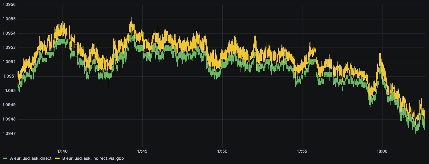
When plotting the direct and indirect rates, we can see that the indirect cost is, unsurprisingly, highly correlated to the direct rate. However, we can also see that the indirect rate always has an offset.

This is easy to understand intuitively. By buying EUR directly against the USD, we only conduct one transaction and cross the spread on EURUSD only.

When doing this via GBP, we need to cross the spread twice:

1. on EURGBP
2. on GBPUSD

This results in higher trading costs and means arbitrage opportunities are even sparser.

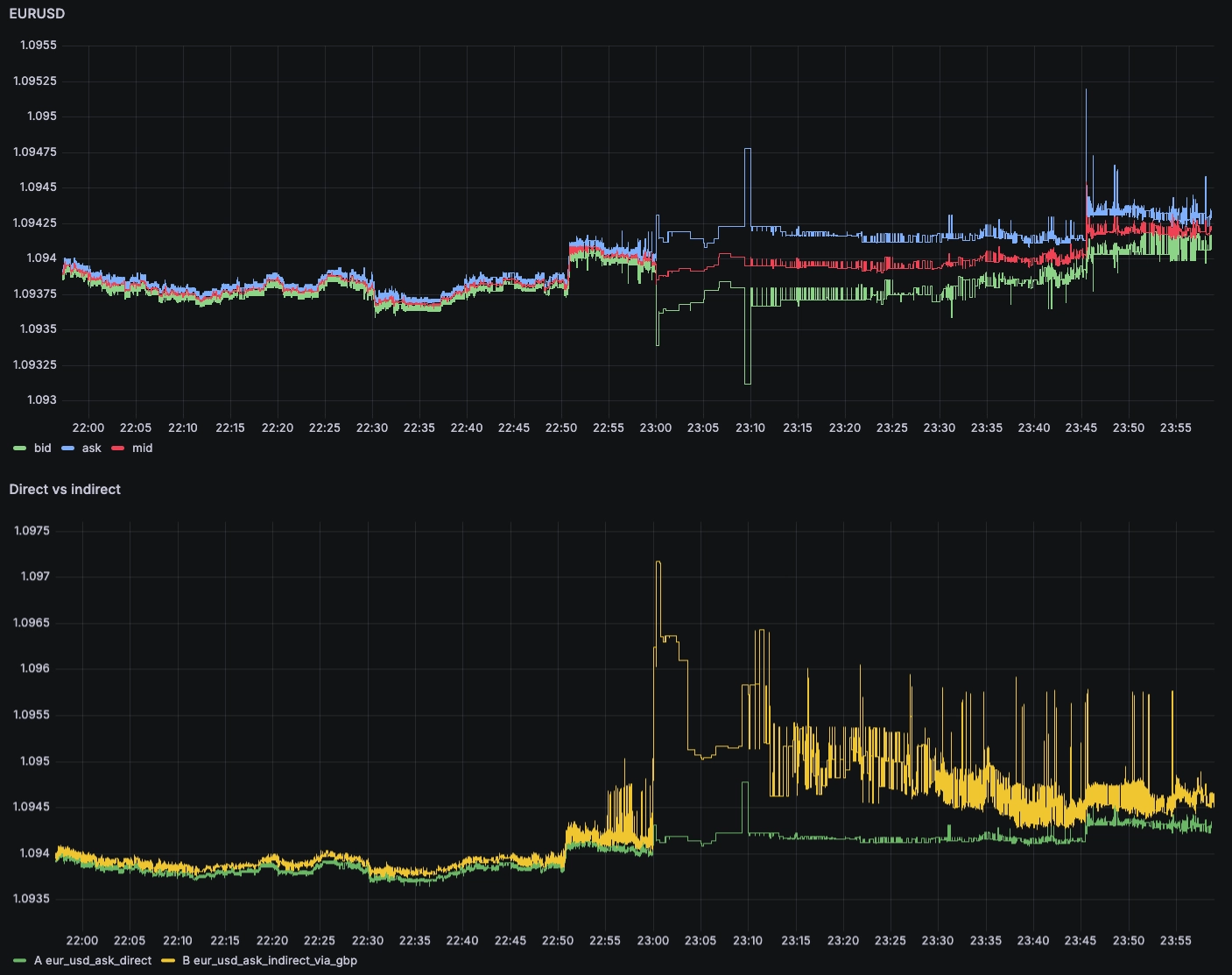
We can see this offset increase sharply after 23:00. This likely corresponds to the overnight period, between US close and Asian open. All currencies continue trading between dealers, which is why we continue seeing quotes, but some dealers probably turn off quoting or increase spreads in this less liquid period.

But below, we can see in the first chart how the spreads widen at 23:00 exactly. In the second chart, we see how this greatly increases the cost of trading indirectly (i.e., crossing the book twice) compared to a direct trade on the pair.

Spread analysis

Since we're talking about spread, we can use the new spread_bps to get an idea of how tight the pairs are trading, and how this changes over time.

The spread_bps function is more syntactic sugar which allows for simple queries. Without spread_bps() and mid(), a user would need to write something like 10000 * (ask - bid) / ((bid + ask) / 2) to yield the same result. With them, we can greatly simplify the query:

SELECT timestamp, pair, avg(spread_bps(bid, ask)) spread_bps 
FROM fxrates 
SAMPLE BY 10s

In this instance, we can see a few things. The first is that EURUSD is very liquid (around 0.6 bps spread) whereas EURGBP and GBPUSD are closer to 0.9 or 1 bps.

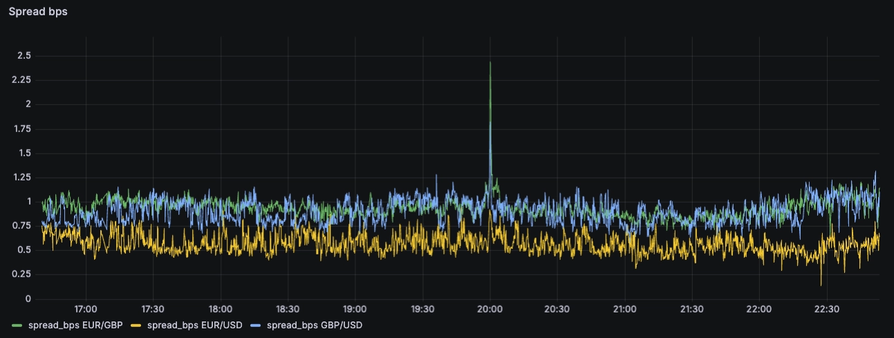
While these spreads are mostly static during the day, we can see the 'overnight' increase again when zooming out to a full day.

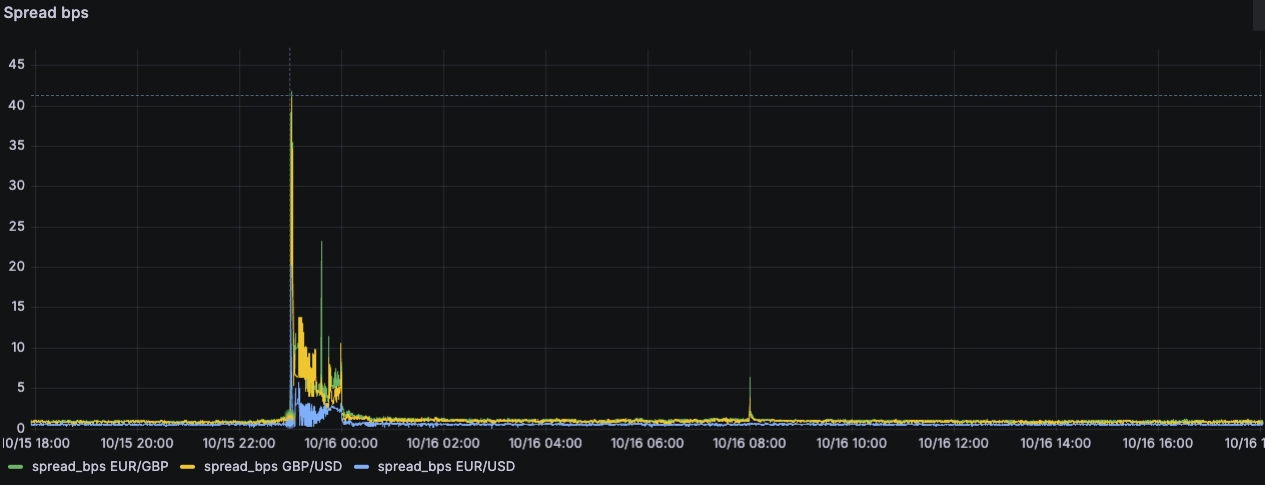
This increase in spread seems to correlate with the daily one-hour close of the CME Currency futures.

Quite possibly, fewer dealers in the OTC markets at these hours, combined with the daily interruption of what is likely one of the only sources of price discovery at this time causes this increase in spread, not the best time to exchange currencies!

Another thing we can note on the above chart is the spike at 8 am which correlates with the European market open. However, when we look at other dates, we don't see this spike happening consistently.

We can run the following query to see if any trend exists (e.g., spread increase at US or European open):

SELECT hour, avg FROM (
SELECT day(timestamp), hour(timestamp), avg(spread_bps(bid,ask)) 
FROM fxrates WHERE pair = 'EUR/GBP' 
ORDER BY day asc, hour asc)

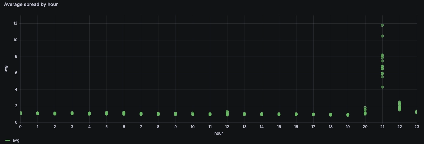
However, besides the overnight widening, there does not seem to be a persistent widening of the FX pairs in scope at other times of the day with the exception of the overnight period.

Looking at regressions and correlations

The new regr_slope function allows us to calculate the slope of the linear regression for two variables. In the below query, we can look at the relationship of EURUSD (the dependent variable) with GBPUSD (the independent variable).

The query makes use of SAMPLE BY to calculate aggregates, in this case on one-minute intervals, of the regression slope:

WITH
eurusd AS (select timestamp, mid(bid, ask) eurusd FROM fxrates WHERE pair = 'EUR/USD'),
gbpusd AS (select timestamp, mid(bid, ask) gbpusd FROM fxrates WHERE pair = 'GBP/USD')
SELECT eurusd.timestamp, regr_slope(eurusd, gbpusd) FROM eurusd ASOF JOIN gbpusd
WHERE $__timeFilter(eurusd.timestamp)
SAMPLE BY 1m

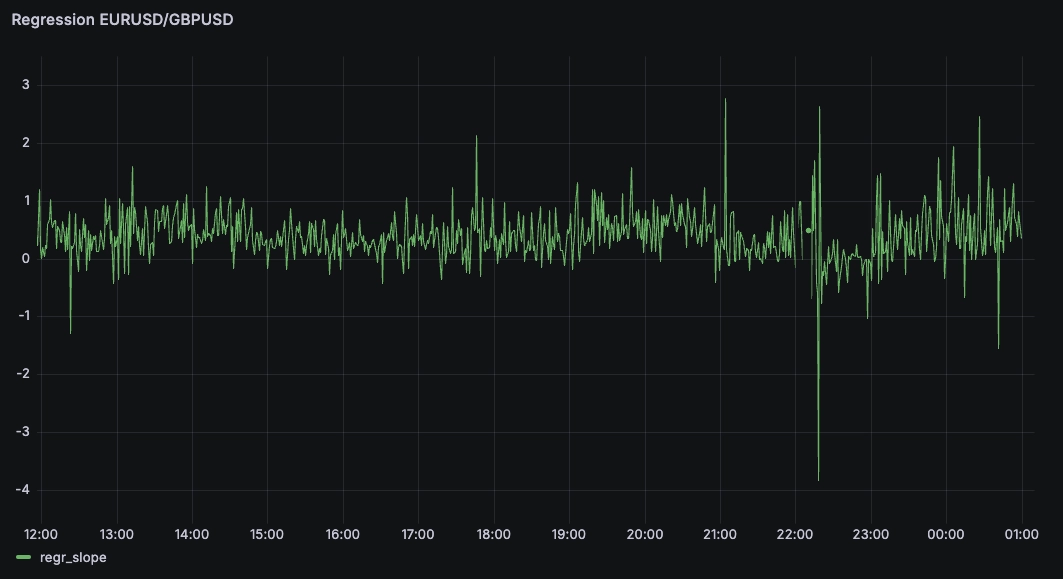
By eyeballing it, the slope over the selected day seems to be around +0.5 which means for any 1% increase of GBPUSD, EURUSD increases by 0.5%. However, one limitation of this is that the slope is only the best fit.

It does not give us an estimate of how well this fits. One way to get an intuitive understanding of how significant the correlation is would be to calculate the coefficient of determination.

One thing we can do is get a feel for it is to plot the two performances on a Grafana XY chart. We can again resort to ASOF JOIN to stitch both currencies performance on the same time axis:

WITH
eurusd AS (SELECT timestamp, last(mid(bid,ask))/first(mid(bid,ask)) -1 p1 FROM fxrates WHERE pair = 'EUR/USD' SAMPLE BY 1m),
gbpusd AS (SELECT timestamp tp, last(mid(bid,ask))/first(mid(bid,ask)) -1 p2 FROM fxrates WHERE pair = 'GBP/USD' SAMPLE BY 1m)
SELECT timestamp, p1 eur_usd, p2 gbp_usd FROM eurusd ASOF JOIN gbpusd
WHERE $__timeFilter(timestamp)

This yields the following plot:

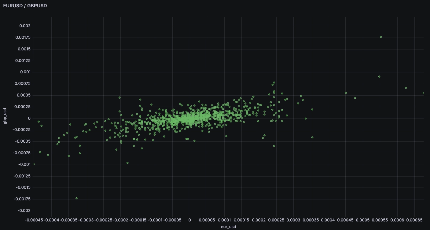
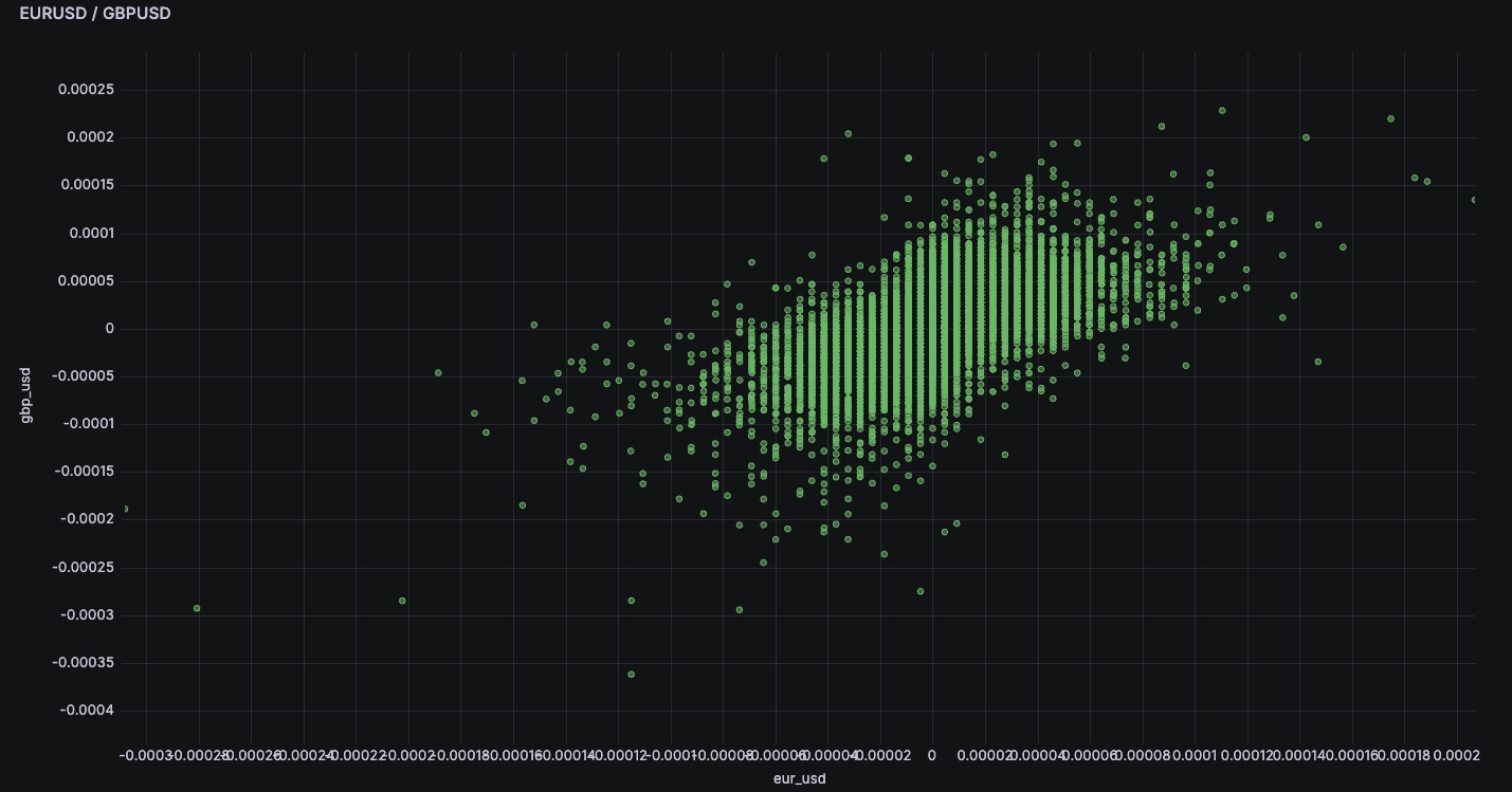
Given the granularity of the dataset, we can look at the correlation for even shorter time frames, for example by changing the SAMPLE BY parameter from 1m to 1 second. This yields the following scatter. It seems much less concentrated than the previous one because it incorporates much more noise due to the higher sampling frequency:

Conclusion

This high-resolution dataset is pretty neat because it contains quite a lot of updates and gives a solid feel for what high-frequency data can look like. Such resolution enables us to run quite a range of analyses on diverse time frames, from minutes/hours to sub-second. While we only touched the surface to showcase some of the new functions, we hope it will inspire some to dig into these datasets as they are fascinating to look at.

For more financial blogs, checkout:

• Scaling trading bot with time-series database
• Making a trading gameboy
• Stories in French real estate data
• Ingesting financial tick data using a time-series database
• Ingesting live market data from DataBento
• Analyzing Bitcoin options data