osthread()->thread_id();
char *s;
char stat[2048];
size_t statlen;
char proc_name[64];
int count;
long sys_time, user_time;
char cdummy;
int idummy;
long ldummy;
FILE *fp;
os::snprintf_checked(proc_name, 64, "/proc/self/task/%d/stat", tid);
fp = os::fopen(proc_name, "r");
if (fp == nullptr) return -1;
statlen = fread(stat, 1, 2047, fp);
stat[statlen] = '\0';
fclose(fp);
// Skip pid and the command string. Note that we could be dealing with
// weird command names, e.g. user could decide to rename java launcher
// to "java 1.4.2 :)", then the stat file would look like
// 1234 (java 1.4.2 :)) R ... ...
// We don't really need to know the command string, just find the last
// occurrence of ")" and then start parsing from there. See bug 4726580.
s = strrchr(stat, ')');
if (s == nullptr) return -1;
// Skip blank chars
do { s++; } while (s && isspace((unsigned char) *s));
count = sscanf(s,"%c %d %d %d %d %d %lu %lu %lu %lu %lu %lu %lu",
&cdummy, &idummy, &idummy, &idummy, &idummy, &idummy,
&ldummy, &ldummy, &ldummy, &ldummy, &ldummy,
&user_time, &sys_time);
if (count != 13) return -1;
return (jlong)user_time * (1000000000 ...
### QuestDB 9.3: Window joins, views, PIVOT, and AI in the console
**URL**: https://questdb.com/blog/questdb-9-3-release/
**Description**: QuestDB 9.3 introduces window joins for range-based time alignment, views for reusable query logic, PIVOT for wide-schema aggregations, and AI-assisted workflows directly inside the Web Console.
Happy new year! Time to update those `WHERE timestamp IN '2025'` filters.
We are kicking off the year with QuestDB 9.3, which packs four major additions:
**window joins** for correlating rows with aggregates from a surrounding time
range, **views** for reusable query logic with overridable parameters,
**PIVOT** to reshape rows into columns, and **AI assistance** built into the
Web Console using your own API keys.
Let us walk through each one.
---
Window joins: range-based time alignment
Time-series analytics often require correlating events with data from a
surrounding time window, for example looking at market prices around each
trade, or sensor readings before and after an anomaly.
Previously, you would need complex subqueries or correlated joins to answer
questions like "what was the average price in the 10 seconds after each trade?"
QuestDB 9.3 introduces [window joins](/docs/query/sql/window-join/), a specialized join syntax for exactly
this pattern. Each row from a primary table joins with a time window of rows
from another table, and aggregations are computed over the matching rows.
Note this is an initial release of Window Joins, which will be improved at the upcoming 9.3.1 release.
Example: trades and surrounding prices
Consider an FX trading scenario where you want to correlate each trade with
the average bid and ask prices from the 10 seconds following the trade:
```questdb-sql title="Window join on trades and prices"
SELECT
t.*,
avg(p.bid_price) AS avg_bid,
avg(p.ask_price) AS avg_ask,
min(p.timestamp) AS from_ts,
max(p.timestamp) AS to_ts
FROM fx_trades t
WINDOW JOIN core_price p ON symbol
RANGE BETWEEN 0 seconds FOLLOWING AND 10 seconds FOLLOWING
INCLUDE PREVAILING
WHERE t.timestamp IN today();
```
The `RANGE BETWEEN ... FOLLOWING` clause defines the time window relative to
each trade. `INCLUDE PREVAILING` ensures you get the most recent price even if
there is no exact match at the window boundary.
This eliminates pag...
### QuestDB 2025: Year in Review
**URL**: https://questdb.com/blog/questdb-2025-year-in-review/
**Description**: 16 open-source releases and 15 enterprise releases: arrays, nanosecond timestamps, DECIMAL, optimized joins, and enterprise replication. From capital markets to crypto, fintech, and high-cardinality sensor workloads.
2025 was transformative for QuestDB. Across 16 open-source releases and 15 enterprise releases, we shipped features for the most demanding time-series workloads.
Capital markets remains our deepest focus. Trading desks, quants, algo traders, and market makers drove features like arrays for order book analytics, nanosecond timestamps for fuller time resolution, DECIMAL for exact calculations, optimized joins for TCA, and enterprise-grade replication.
But we're also seeing strong adoption beyond finance. DECIMAL is critical for crypto where tracking Bitcoin balances requires high precision. Ingestion robustness and high throughput for high-cardinality workloads serve energy, aerospace, and PhysicalAI/Robotics teams handling millions of distinct sensor series. And QPS and latency optimizations power fraud detection across fintech and crypto/web3.
We've also invested in open formats. Parquet support enables seamless interoperability with the broader data ecosystem, with more to come in 2026.
Here's what we shipped in 2025.
Data Types: Precision Meets Performance
Capital markets data comes in shapes that traditional databases struggle with. We needed types that match how financial data actually works.
Arrays: Order Books Without Reshaping
**Release**: 9.0 (July 2025)
Order book snapshots are inherently multidimensional: 50-100 bid levels, 50-100 ask levels, each with price and size. Traditionally, you'd flatten this into separate rows, destroying the semantic relationship and making queries painful.
QuestDB 9.0 introduced true N-dimensional arrays with NumPy-like operations and zero-copy performance. Now you can store complete order book snapshots as native array columns:
```sql
CREATE TABLE orderbook_snapshots (
timestamp TIMESTAMP,
symbol SYMBOL,
bids DOUBLE[][], -- [price, size] pairs
asks DOUBLE[][] -- [price, size] pairs
) TIMESTAMP(timestamp) PARTITION BY DAY;
```
Query the entire order book history without reshaping. Compute cumulative d...
### Benchmark and comparison: QuestDB vs. ClickHouse
**URL**: https://questdb.com/blog/clickhouse-vs-questdb-comparison/
**Description**: Benchmarks and an overview of ClickHouse versus QuestDB to compare features, functionality, performance, and ease of use.
ClickHouse is one of the most widely used analytical databases. It started at Yandex for web analytics and now runs observability, product analytics and general OLAP at very large scale, with a broad ecosystem behind it. QuestDB is the leading time-series database for streaming ingestion and low-latency queries, used for mission-critical workloads where throughput is high and data cannot be lost, capital markets first among them. Teams looking for a fast analytical engine often end up evaluating both.
ClickHouse is the broader analytical database. QuestDB is the database for the live, authoritative event record: rows arrive continuously, none of them can be lost, and the same SQL engine serves the newest state in milliseconds and years of history. Choose ClickHouse for log monitoring and observability, product analytics, semi-structured data and general OLAP. Choose QuestDB for the data a business runs on: market data and trades, telemetry from an energy plant, a rocket or a fleet of robots, where a single lost record has consequences.
This article runs the two through the same TSBS benchmark on the same machine, ClickHouse 26.7.5.10 against QuestDB 9.3.3, publishes every number, and then looks at where they differ in architecture and focus.
```info
These benchmarks predate QWP, the binary protocol we shipped in
[QuestDB 10.0](/blog/questdb-10-release/) in August 2026. Ingestion here runs
over InfluxDB Line Protocol, a text format the server parses row by row. QWP
sends binary columns instead, up to
[3.6x faster over a network](/blog/qwp-vs-ilp-ingestion-benchmark/), and it
[streams reads back as Arrow](/blog/streaming-500-million-rows-into-apache-arrow/).
Read the QuestDB figures below as a floor.
```
Two databases, different strengths
**QuestDB** is built for streaming ingestion and low-latency queries, at any batch size from a single row up. It came out of trading floors, eFX desks at tier-1 banks, and today sits on the critical path in trading, defense, ene...
### How to Build Market Depth Charts from Order Book Data with QuestDB
**URL**: https://questdb.com/blog/analyzing-market-depth-questdb/
**Description**: Learn how to model FX order book data in QuestDB using SQL arrays and build real-time market depth charts for trading and market microstructure analysis.
If you've ever looked at a trading terminal or watched market data flow by, you've probably noticed those waterfall-like
charts showing layers of buy and sell orders stacked at different price levels. These are market depth charts, and
they're one of the most valuable tools for understanding what's really happening in a market at any given moment.
In this post, I'll walk through how to store order book data efficiently in QuestDB using arrays, and then show you how
to transform that data into market depth visualizations using SQL. By the end, you'll understand not just how to build
these charts, but why they matter for anyone working with financial data. In fact, the techniques we'll cover here are
exactly what power the market depth chart (top right panel) in our [live FX order book dashboard](https://questdb.com/dashboards/fx-orderbook/),
which visualizes real-time EUR/USD, GBP/USD, and other major currency pairs.
Understanding Order Books and Market Depth Charts
Before we dive into the technical implementation, let's talk about what we're actually modeling here. If you're already
familiar with order books and market making, feel free to skip ahead. But if terms like "best bid" and "order book levels"
sound like financial jargon, stick with me for a moment.
The Order Book: A Market's Memory
An order book is essentially a live snapshot of supply and demand for a financial instrument. Think of it as a two-sided
auction that never stops. On one side, you have buyers (the "bid" side) saying "I want to buy at this price." On the other
side, you have sellers (the "ask" or "offer" side) saying "I'll sell at this price."
Each side of the book is organized by **price levels**. A price level is simply a price point where one or more orders are
waiting. For example, if three different traders want to buy EUR/USD at 1.1650, that becomes one price level with the combined
volume from all three orders.
Here's where it gets interesting: the bid side is sorted in **descendi...
### How a Kernel Bug Froze My Machine: Debugging an Async-profiler Deadlock
**URL**: https://questdb.com/blog/async-profiler-kernel-bug/
**Description**: How I investigated and worked around a kernel bug that caused async-profiler to freeze my machine whenever I tried to use a profiler.
I've been a Linux user since the late 90s, starting with [Slackware](http://www.slackware.com/) on an underpowered AMD K6.
Over the years I've hit plenty of bugs, but the last decade has been remarkably stable - until a kernel bug started
freezing my machine whenever I used [async-profiler](https://github.com/async-profiler/async-profiler/).
I'm not a kernel developer, but I found myself poking around kernel source code to understand the problem better and
figure out what was going on under the hood.
The problem
I was about to start an investigation of latency spikes in QuestDB reported by a user. To do that, I wanted to use the async-profiler to capture [CPU heatmaps](https://github.com/async-profiler/async-profiler/blob/3a493bedc4c6463ba19970018c50e0c9d7dcbfda/docs/Heatmap.md).
However, when I tried to attach the profiler, my machine froze completely. It did not respond to any
keys, it was impossible to switch to a terminal, it did not respond to SSH. The only way to recover was to hard
reboot it. I tried to start QuestDB with the profiler already configured to start at launch - the same result, a frozen machine almost immediately after the launch.
I thought that was weird, this had not happened to me in years. It was already late in the evening, I felt tired anyway so I decided to call it a day. There was a tiny chance I was hallucinating
and the problem would go away by itself overnight. A drowning man will clutch at a straw after all.
The next day, I tried to attach the profiler again - same result, frozen machine. Async-profiler integration in QuestDB is a relatively new feature, so I thought
there might be a bug in the integration code, perhaps a regression in the recent QuestDB release. So I built an older QuestDB version: The same result, frozen machine. This was puzzling - I positively
knew this worked before. How do I know? Because I worked on the [integration code](https://github.com/questdb/questdb/pull/6150) not too long ago, and I tested t...
### InfluxDB 3 Core Benchmarks: QuestDB Comparison
**URL**: https://questdb.com/blog/influxdb3-core-benchmarks/
**Description**: Performance benchmarks comparing InfluxDB 3 Core against QuestDB 9.3.3 using the industry-standard TSBS benchmark suite.
This article benchmarks InfluxDB 3 Core against QuestDB 9.3.3. InfluxDB 3 Core, which [reached general availability in April 2025](https://www.businesswire.com/news/home/20250415573560/en/InfluxData-Announces-General-Availability-of-InfluxDB-3-Core-and-InfluxDB-3-Enterprise-Simplifying-How-Developers-Build-with-Time-Series-Data), is a complete rewrite of InfluxDB using Apache Arrow and DataFusion.
**Key results:** QuestDB ingests 7 to 8.6 million rows per second at every cardinality we tested; InfluxDB 3 Core holds a flat 319K. On queries, InfluxDB 3 Core is slower than QuestDB on every type and slower than InfluxDB v1 and v2 on most. Simple one-hour aggregations take around 55 ms against QuestDB's sub-millisecond, and the full-table scan is the one place the two are close, 1.24 s against 1.03 s.
> **For InfluxDB v1/v2 benchmarks and detailed architecture comparison, see [QuestDB vs InfluxDB](/blog/influxdb-vs-questdb-comparison/)**.
```info
These benchmarks predate QWP, the binary protocol we shipped in
[QuestDB 10.0](/blog/questdb-10-release/) in August 2026. Ingestion here runs
over InfluxDB Line Protocol, a text format the server parses row by row. QWP
sends binary columns instead, up to
[3.6x faster over a network](/blog/qwp-vs-ilp-ingestion-benchmark/), and it
[streams reads back as Arrow](/blog/streaming-500-million-rows-into-apache-arrow/).
Read the QuestDB figures below as a floor.
```
About InfluxDB 3 Core
InfluxDB 3 Core represents a major architectural shift for InfluxDB:
- **Complete rewrite** in Rust (previously Go)
- **Apache Arrow** for in-memory data representation
- **DataFusion** query engine (Apache Arrow's SQL query engine)
- **Parquet** for storage format
- **Arrow Flight** for query protocol (gRPC-based)
It is a different database from v1 and v2, built around columnar processing for analytical queries.
Performance benchmarks
We use the open-source, industry-standard [Time Series Benchmark Suite (TSBS)](https://github.com/questdb/tsbs)...
### Benchmark and comparison: QuestDB vs. InfluxDB v1/v2
**URL**: https://questdb.com/blog/influxdb-vs-questdb-comparison/
**Description**: Benchmarks and an overview of InfluxDB versus QuestDB to compare features, functionality, performance, and ease of use.
InfluxDB is one of the most widely used time-series databases. InfluxData released it in 2013 for metrics and monitoring, with Telegraf as the collector and a measurement-and-tag model that made dashboards over server and application metrics easy. v1 and v2 run on the TSM engine; InfluxDB 3 is a ground-up rewrite with a different storage and query engine and has [its own comparison](/blog/influxdb3-core-benchmarks/). QuestDB is the leading open-source time-series database for streaming ingestion and low-latency queries. It came out of trading floors and sits on the critical path in trading, defense, energy and robotics systems, where throughput is high and data cannot be lost.
The difference comes down to what happens if data is lost. InfluxDB is built for monitoring, where data gets downsampled over time and a few lost points don't matter. QuestDB is for the data that cannot be lost: the full-fidelity operational record, with the newest state available in milliseconds, years of history behind it, and one SQL engine across all of it.
Choose InfluxDB for infrastructure monitoring, Telegraf pipelines and dashboards over a known set of series. Choose QuestDB when the data is mission critical.
This article runs InfluxDB v1.12.4, InfluxDB v2.9.1 and QuestDB 9.3.3 through the same TSBS workload on the same machine, publishes every result, and shows where the architectural difference starts to matter.
**Key results:** QuestDB ingests 7 to 8.6 million rows per second at every cardinality we tested, while InfluxDB falls from 1.1 million to under 240K as hosts increase. InfluxDB v1 is faster on the narrowest single-host queries; QuestDB is faster on every query that aggregates across hosts, by a wide margin.
```info
These benchmarks predate QWP, the binary protocol we shipped in
[QuestDB 10.0](/blog/questdb-10-release/) in August 2026. Ingestion here runs
over InfluxDB Line Protocol, a text format the server parses row by row. QWP
sends binary columns instead, up to
[3.6...
### TimescaleDB vs QuestDB: 2026 Benchmark Results
**URL**: https://questdb.com/blog/timescaledb-vs-questdb-comparison/
**Description**: Compare QuestDB and TimescaleDB with up-to-date performance benchmarks and architectural comparisons.
TimescaleDB and QuestDB are both open-source time-series databases. TimescaleDB
is a PostgreSQL extension that adds time-series storage and functions to a
database many teams already run. QuestDB is a standalone engine built for
ingestion throughput and query latency.
TimescaleDB is the right choice when you already run PostgreSQL and want time series inside it. You keep your drivers and tooling and get hypertables and continuous aggregates on top. QuestDB is for the workloads PostgreSQL was never built for. It ingests millions of rows a second and serves the latest state in milliseconds with years of history behind it, for the cases where a single lost record has consequences.
This article runs both through the same TSBS benchmark on the same machine, TimescaleDB 2.29.1 against QuestDB 9.3.3, publishes every number, and then looks at the architectural differences behind
the results.
```info
These benchmarks predate QWP, the binary protocol we shipped in
[QuestDB 10.0](/blog/questdb-10-release/) in August 2026. Ingestion here runs
over InfluxDB Line Protocol, a text format the server parses row by row. QWP
sends binary columns instead, up to
[3.6x faster over a network](/blog/qwp-vs-ilp-ingestion-benchmark/), and it
[streams reads back as Arrow](/blog/streaming-500-million-rows-into-apache-arrow/).
Read the QuestDB figures below as a floor.
```
Introducing TimescaleDB & QuestDB
DB-Engines classifies them like this:
| Feature | QuestDB | TimescaleDB |
| ----------------------- | ------------------------- | ----------------- |
| Primary database model | Time Series DBMS | Time Series DBMS |
| Implementation language | Java (zero-GC), C++, Rust | C |
| SQL? | Yes | Yes |
| APIs | QWP, ILP, HTTP, PGWire, JDBC | JDBC, ODBC, C lib |
TimescaleDB is a time series database built atop PostgreSQL. It's provided under
two li...
### We finally benchmarked InfluxDB 3 OSS Core (Alpha)
**URL**: https://questdb.com/blog/influxdb3-core-alpha-benchmarks-and-caveats/
**Description**: We benchmark InfluxDB 3 OSS Core (Alpha) ingestion against QuestDB, take an initial look at its strengths and weaknesses, and flag key caveats.
> **Editor’s note:** This article was written during the InfluxDB 3 alpha phase. InfluxDB 3 is now generally available. For up-to-date benchmarks and performance comparisons against QuestDB, see our latest [InfluxDB 3 Core benchmark](https://questdb.com/blog/influxdb3-core-benchmarks/).
```info
These benchmarks predate QWP, the binary protocol we shipped in
[QuestDB 10.0](/blog/questdb-10-release/) in August 2026. Ingestion here runs
over InfluxDB Line Protocol, a text format the server parses row by row. QWP
sends binary columns instead, up to
[3.6x faster over a network](/blog/qwp-vs-ilp-ingestion-benchmark/), and it
[streams reads back as Arrow](/blog/streaming-500-million-rows-into-apache-arrow/).
Read the QuestDB figures below as a floor.
```
InfluxDB 3 released as a [Cloud-only product](https://www.influxdata.com/blog/introducing-influxdb-3-0/) in April 2023.
Along with the release, the team announced their plans to [release an open source version](https://www.influxdata.com/blog/the-plan-for-influxdb-3-0-open-source/).
It was billed as having 100x faster queries, 10x faster ingestion performance, and 10x better compression.
The community was enthusiastic, especially for the release of the open source version.
At long last, in January 2025, InfluxDB 3 Core Alpha [finally released](https://www.influxdata.com/blog/influxdb3-open-source-public-alpha/).
The release blog post states it is "a high-performance recent-data engine". This is a slight deviation from the usual "time-series database" descriptor, and we'll unpack precisely why.
But before we get too deep, we should mention that InfluxData states that version 3 is Alpha and **not production-ready**.
Given it's working in their cloud, and that we didn't want to wait for a stable version to get a ballpark of its performance,
we decided to offer an early look.
In our testing, we found that InfluxDB 3.0 Core ingested data approximately **5.5 times slower** than QuestDB 8.2.2.
We'll unpack the resu...
### QuestDB 9.2: Exact arithmetic and smarter temporal joins
**URL**: https://questdb.com/blog/questdb-9-2-release/
**Description**: QuestDB 9.2 introduces a native DECIMAL type for exact arithmetic, a new Dense ASOF JOIN algorithm for long distance temporal matches, and quality of life improvements like symbol auto scaling enabled by default.
With QuestDB 9.2, you get native [decimals](/docs/query/datatypes/decimal/) for exact arithmetic and a faster engine for temporal joins.
This release introduces a new **DECIMAL** type for precise numeric work, a [**Dense ASOF JOIN** algorithm](/docs/concepts/deep-dive/sql-optimizer-hints/#dense-algo)
for workloads with long distance matches, and makes **symbol capacity auto scaling** the default so
high cardinality datasets work smoothly.
If 9.0 armed QuestDB with arrays and 9.1 added nanosecond timestamps and continuous profiling, 9.2
is about getting your numbers and temporal joins exactly right.
Let us dive in.
---
Exact arithmetic with DECIMAL
Fixed-point arithmetic is great for physics, not so great for ledgers.
If you have ever seen `0.30000000000000004` in a financial report, you know the problem. Floating
point types like `DOUBLE` trade a bit of numerical accuracy for speed and range. That is usually
fine, but not when you are reconciling accounts, PnL, or crypto balances.
QuestDB 9.2 introduces a native `DECIMAL(precision, scale)` [type](/docs/query/datatypes/overview/) that stores fixed point numbers
with **exact arithmetic**.
```questdb-sql title="Floating point vs DECIMAL"
-- With DOUBLE:
SELECT 0.1 + 0.2;
-- With DECIMAL:
SELECT 0.1m + 0.2m;
```
- The first query uses `DOUBLE` and can produce `0.30000000000000004`.
- The second uses DECIMAL literals (the `m` suffix) and returns `0.3` exactly.
No hidden rounding, no surprises.
Precision and scale, without thinking about storage
`DECIMAL` follows the classic SQL model:
- `precision` is the total number of significant digits.
- `scale` is how many digits live after the decimal point.
For example, `DECIMAL(14, 2)` gives you up to 999,999,999,999.99, which is usually enough for
monetary amounts in a single currency.
```questdb-sql title="Defining financial columns with DECIMAL"
CREATE TABLE transactions (
id LONG,
account_id SYMBOL,
amount DECIMAL(14, 2), -- up to ...
### Building an FX Liquidity Stress Analysis Workflow with QuestDB
**URL**: https://questdb.com/blog/fx-liquidity-stress-analysis-workflow-questdb/
**Description**: Build an FX liquidity stress pipeline with QuestDB: ingest L2 order book data, engineer features, label stress, and train an XGBoost model
Liquidity dry-ups in FX markets can sharply raise execution costs for large
institutional orders. During stressed conditions, bid–ask spreads widen and
market depth thins out, making it harder to execute large trades efficiently.
Traditional indicators often react only after the fact, so traders have little
time to adjust.
In this tutorial, we build a compact FX liquidity stress analysis pipeline using
QuestDB and Python. We’ll show how to stream and aggregate high-frequency order
book data, engineer microstructure features, label stress periods, and train an
XGBoost model for early warnings. The focus is on reproducible data science, not
black-box trading: everything runs end-to-end with open tools and SQL-based
time-series processing.
The Liquidity Challenge in FX Markets
Episodes of stress in FX markets often emerge without warning. The
[IMF reports](https://www.imf.org/en/Blogs/Articles/2025/10/07/economic-uncertainty-can-test-the-resilience-of-the-foreign-exchange-market)
that during periods of uncertainty,
> currency bid-ask spreads widen, and foreign funding and hedging costs rise.
These conditions typically appear around macro announcements, flash crashes, or
when major trading sessions overlap and liquidity providers withdraw. As order
book depth evaporates, execution costs can spike within seconds.
Conventional monitoring tools only register these shifts once spreads have
already widened. Understanding and anticipating such moments requires data with
fine time resolution, showing how spreads, volumes, and imbalance evolve in the
seconds before stress appears. In this workflow we use second-level aggregated
data for simplicity, but the same ideas apply to sub-second or microsecond
feeds.
Detecting stress ahead of time involves two main ingredients:
- Computing liquidity measures such as spread,
[imbalance](/glossary/order-book-imbalance/), depth, and volatility on
streaming market data.
- Training a model on historical patterns to identi...
### The Mystery of the Phantom Quote in My CI Builds
**URL**: https://questdb.com/blog/azure-pipelines-stdout-stderr-race-condition/
**Description**: How a phantom single quote from bash's set -x caused random CI build failures through a race condition between stdout and stderr in Azure Pipelines.
Working on distributed systems at Hazelcast and now at QuestDB, I've debugged my share of race conditions - the kind involving network partitions,
timing issues, and subtle concurrency bugs. But the bug I hit last week was different.
A CI build was failing randomly, all because of a single, phantom single-quote ('). The root cause? Not a typo,
not a dangling string, but a bizarre race condition... **between stdout and stderr**.
The Setup: A "Simple" CI Step
My goal was straightforward: speed up our Rust builds in Azure Pipelines using [`sccache`](https://github.com/mozilla/sccache/). The plan was simple:
1. Create a Bash script step to run on our macOS and Windows builders.
2. The script would check if `sccache` was already installed.
3. If not, it would download the correct release from GitHub, unpack it, and move it to a known path.
4. Finally, it would set the `RUSTC_WRAPPER` environment variable for subsequent steps using the `##vso[task.setvariable]` [logging command](https://learn.microsoft.com/en-us/azure/devops/pipelines/process/set-variables-scripts?view=azure-devops&tabs=bash).
> A quick note on `##vso[task.setvariable]`: This is an Azure Pipelines logging command - a special string that the agent watches for in your script's output (on both stdout and stderr). When it sees this pattern, it parses the command and sets an environment variable that subsequent steps in the pipeline can use. It's how you pass values between different tasks in a pipeline. You simply echo the command, and the agent does the rest.
Here's what the pipeline step looked like:
```yaml
- bash: |
set -eux
SCCACHE_VERSION="0.10.0"
export PATH="$(CARGO_INSTALL_PATH)/bin:$PATH"
if [ "$(uname)" == "Darwin" ]; then
SCCACHE_BINARY="sccache"
ARCHIVE="sccache-v${SCCACHE_VERSION}-x86_64-apple-darwin.tar.gz"
else
SCCACHE_BINARY="sccache.exe"
ARCHIVE="sccache-v${SCCACHE_VERSION}-x86_64-pc-windows-msvc.tar.gz"
fi
if [ -f "$(CARGO_...
### Order Book Imbalance Analysis with QuestDB Arrays
**URL**: https://questdb.com/blog/order-book-imbalance-analysis/
**Description**: Analyze order book imbalance with QuestDB array types, using synthetic Bitcoin data for metrics, queries, and Grafana views to spot spoofing and price pressure.
```info
For a related quote-based metric, see the
[Order Flow Imbalance cookbook recipe](/docs/cookbook/sql/finance/order-flow-imbalance/).
```
Order Book Imbalance Analysis with QuestDB Arrays
[Order book imbalance](/glossary/order-book-imbalance/) (OBI) is a simple yet powerful metric that
measures the disparity between buy and sell orders at different price points in an order book.
OBI provides insight into short-term price pressure that often leads to directional moves, making
it an early indicator for traders looking to capitalize on market movements.
Storing order book data to compute OBI with traditional relational databases has been challenging
as you need to use multiple columns to store bid/ask prices and bid/ask volumes at each price level.
A sample schema to capture that market data may look like the following:
```questdb-sql
CREATE TABLE market_data (
timestamp TIMESTAMP,
symbol SYMBOL,
bid_price_1 DOUBLE, bid_volume_1 DOUBLE,
bid_price_2 DOUBLE, bid_volume_2 DOUBLE,
ask_price_1 DOUBLE, ask_volume_1 DOUBLE,
ask_price_2 DOUBLE, ask_volume_2 DOUBLE,
) TIMESTAMP(timestamp) PARTITION BY HOUR;
```
Then you would need to aggregate those columns to calculate total liquidity and calculate other
metrics for further analysis. With QuestDB 9.0, representing this data has become significantly
easier with N-dimensional array types. Instead of storing each price and volume level in separate
columns, you can store them in NumPy-like arrays and make use of array functions like `array_avg`,
`array_sum`, `array_count`, and `array_stddev_samp` for simple analysis. In other words, the table
schema can be represented cleanly like the following instead:
```questdb-sql
CREATE TABLE market_data (
timestamp TIMESTAMP,
symbol SYMBOL,
bids DOUBLE[][],
asks DOUBLE[][]
) TIMESTAMP(timestamp) PARTITION BY HOUR;
```
In this tutorial, let’s take a look at analyzing order book imbalance using synthetic Bitcoin data.
You can follow along by downloading the s...
### QuestDB 9.1: Precision, Profiling, and Power
**URL**: https://questdb.com/blog/questdb-9-1-release/
**Description**: QuestDB 9.1 brings nanosecond timestamps, continuous profiling, dynamic symbol map scaling, and major JOIN and performance improvements. It is our most precise and introspective release yet.
QuestDB 9.1 is here. Precision and introspection meet performance.
This release introduces **nanosecond timestamps**, integrated **continuous profiling**,
**auto-scaling symbol maps**, and **smarter JOINs**. The result: more precision, more visibility,
and more throughput, all in one release.
Let’s dive in.
---
Nanosecond timestamps
For workloads where every nanosecond counts, QuestDB now supports a new data type:
[`TIMESTAMP_NS`](/docs/query/datatypes/overview/#timestamp-and-date-considerations).
```questdb-sql title="Creating a nanosecond-precision table"
CREATE TABLE ticks (
ts TIMESTAMP_NS,
symbol SYMBOL,
price DOUBLE
) timestamp(ts);
```
- `TIMESTAMP_NS` offers **true nanosecond precision**, ideal for high-frequency trading,
sensor data, or sub-microsecond event tracking.
- The existing `TIMESTAMP` type remains unchanged (microsecond precision).
- You can use `TIMESTAMP_NS` anywhere you would use a regular timestamp, in filters, ordering,
joins, or aggregates.
Backwards compatibility is preserved: older tables continue to use microseconds.
New ones can opt in to nanosecond precision for full analytical accuracy.
```tip
`SAMPLE BY`, `ASOF JOIN`, and window functions all support nanosecond timestamps.
```
---
Continuous profiling
Understanding performance has never been easier.
QuestDB 9.1 integrates the [Async Profiler](https://github.com/questdb/questdb/pull/6150),
the standard low-overhead profiler for the JVM, directly into the server.
You can now capture **CPU or allocation flame graphs** continuously or on demand, without any
external setup.
```bash title="Capture a 30-second CPU profile"
questdb.sh profile -- -e cpu -d 30 -f /tmp/cpu.html
```
Profiles are exported as interactive HTML flame graphs or JFR (Java Flight Recorder) files.
- Zero overhead when idle
- Around 10% overhead when active
- No restart required
Use it to trace slow queries, high CPU usage, or unusual memory patterns, in production or during
load tests....
### QuestDB + Hacktoberfest 2025: Build Something That Lasts
**URL**: https://questdb.com/blog/hacktoberfest-2025-questdb/
**Description**: Join QuestDB for Hacktoberfest 2025. Contribute meaningful pull requests, connect with our community, and earn exclusive swag.
For some, October means cooler nights and early sunsets. For others, it means
longer days and warmer skies. Wherever you are, it is the month when the open
source community comes together to celebrate Hacktoberfest.
At QuestDB we are excited to welcome new and returning contributors to our
projects and to celebrate another year of collaboration.
What is Hacktoberfest?
[Hacktoberfest](https://hacktoberfest.com) is an annual celebration of open
source organized by DigitalOcean. From October 1 through October 31, anyone can
take part by opening pull requests and helping projects grow. It is a great
chance to sharpen your skills and connect with the global developer community.
Why contribute to QuestDB?
QuestDB is an open source time-series database focused on performance and
simplicity. The core engine is built in Java, C++, and Rust. Alongside it we
maintain a web console written in TypeScript and React, and a full set of
documentation. All of these are open for contributions, and Hacktoberfest is the
perfect time to get involved.
We value quality over quantity. Small typo fixes are always appreciated, but for
Hacktoberfest we encourage contributors to look for issues that have a real
impact. You will find open issues with the `hacktoberfest` label in our GitHub
repos. If you are unsure where to begin, drop a message in the **#contributors**
channel of our [Slack](https://slack.questdb.com/) and we will point you in the
right direction. AI-generated contributions are discouraged because we want your
ideas and your work.
Rewards
Contributing to open source is rewarding in itself, but we like to add a little
extra. Anyone who successfully contributes to a QuestDB project during
Hacktoberfest will receive one of our exclusive t-shirts as a thank you. And
that's on top of the [Hacktoberfest Rewards](https://hacktoberfest.com/participation/).
How to get started
1. **Register for Hacktoberfest**: Sign up on the
[official Hacktoberfest website](https://...
### From Rust to Reality: The Hidden Journey of fetch_max
**URL**: https://questdb.com/blog/rust-fetch-max-compiler-journey/
**Description**: Tracing Rust AtomicU64::fetch_max from macro expansion and rustc intrinsics through LLVM atomicrmw umax down to the final x86-64 CAS loop.
How a Job Interview Sent Me Down a Compiler Rabbit Hole
I occasionally interview candidates for engineering roles. We need people who understand
concurrent programming. One of our favorite questions involves keeping track of a
maximum value across multiple producer threads - a classic pattern that appears in many
real-world systems.
Candidates can use any language they want.
In Java (the language I know best), you might write a [CAS loop](https://en.wikipedia.org/wiki/Compare-and-swap),
or if you're feeling functional, use `updateAndGet()` with a lambda:
```java
AtomicLong highScore = new AtomicLong(100);
[...]
highScore.updateAndGet(current -> Math.max(current, newScore));
```
But that lambda is doing work - it's still looping under the hood, retrying if
another thread interferes. You can see the loop right in [AtomicLong's source code](https://github.com/openjdk/jdk/blob/5271448b3a013b2e3edcd619a4a3b975b292dae1/src/java.base/share/classes/java/util/concurrent/atomic/AtomicLong.java#L268-L288).
Then one candidate chose Rust.
I was following along as he started typing, expecting to see either an explicit
CAS loop or some functional wrapper around one. But instead, he just wrote:
```rust
high_score.fetch_max(new_score, Ordering::Relaxed);
```
_"Rust has fetch_max built in,"_ he explained casually, moving on to the next
part of the problem.
Hold on. This wasn't a wrapper around a loop pattern - this was a first-class
atomic operation, sitting right there next to `fetch_add` and `fetch_or`. Java
doesn't have this. C++ doesn't have this. How could Rust just... have this?
After the interview, curiosity got the better of me. Why would Rust provide
`fetch_max` as a built-in intrinsic? Intrinsics usually exist to leverage
specific hardware instructions. But x86-64 doesn't have an `atomic max`
instruction. So there had to be a CAS loop somewhere in the pipeline. Unless...
maybe some architectures _do_ have this instruction natively? And if so, how
does the ...
### Why Parquet Matters for Time Series and Financial Services
**URL**: https://questdb.com/blog/why-parquet-matters-for-time-series-and-finance/
**Description**: Why Parquet fits time-series and financial data: an open columnar format that frees billions of ticks, quotes, and trades from vendor lock-in.
Financial data is growing at a pace that is hard to keep up with. Every tick, quote, and trade across multiple exchanges
adds up fast. A single day can produce billions of rows, and stretch that across months or years, and you are looking at
terabytes of information. Analysts, quants, and data engineers face the same challenge: how do you make sense of all
this data as quick as the market needs it?
[Open formats](/compare/questdb-vs-kdb/#architecture-open-data-vs-proprietary-lock-in) provide the answer. Instead of locking your data into one vendor's ecosystem, open standards let it move
freely. They simplify integration, reduce storage costs, and make pipelines more flexible. No team wants to be stuck
with a rigid system when markets change this quickly.
Among these formats, [Parquet](https://parquet.apache.org/) stands out. By storing data column by column instead of
row by row, Parquet allows you to read only what you need. If your strategy only requires prices and timestamps, you can skip the rest. That means faster queries, lower memory usage, and less unnecessary I/O.
This resonates well with QuestDB, whose mission has always been to provide the fastest time series database. It embraces
open formats, hence it naturally comes with Parquet support.
What Makes Parquet Different
Parquet was originally created at Twitter and Cloudera. Today, it is an Apache project and a standard supported by
nearly every modern analytics tool, including Spark, Flink, DuckDB, Pandas, and, of course, QuestDB.
As mentioned, Parquet is not a "traditional" row-based data format. Row-based storage is like saving it one row at a
time. You grab the whole row, even if you only need a few cells. [Columnar storage](/docs/schema-design-essentials/#columnar-storage-model-and-table-density), such as Parquet or databases
like QuestDB, keeps each column together. When only certain data points are needed, you do not touch the rest.
Parquet has become a standard in the data engineerin...
### Immutable images when embedding QuestDB Java library and noexec /tmp
**URL**: https://questdb.com/blog/questdb-java-noexec-tmp-native-libs/
**Description**: A guide on how to run QuestDB’s Java library in hardened environments where /tmp is mounted with noexec, by pre-bundling native libraries and using the questdb.libs.dir system property.
When `/tmp` is mounted with `noexec` (a common hardening step), the QuestDB **Java** library may still try to unpack its
native libraries into `/tmp` and load them from there. On hardened hosts or minimal containers, this fails with
`UnsatisfiedLinkError` or permission errors.
This guide shows how to run QuestDB’s Java library without writing executables to `/tmp`, by **pre-bundling** the native
libs and pointing QuestDB at them via `-Dquestdb.libs.dir`. It also documents the fallback of redirecting Java’s temp directory.
> **Important:** If you're using **official QuestDB server container images** or **platform-specific distributions**,
you **do not need to do anything**. They already ship the native libraries and set `-Dquestdb.libs.dir`, so nothing gets
unpacked to `/tmp`. The rest of this guide is only for teams building their **own** images from scratch or embedding the
QuestDB Java library in another application.
---
TL;DR
**On official QuestDB images/distributions? You're done. This is already handled.**
* QuestDB’s Java library needs two native libs at runtime:
* `libquestdb.so`
* `libquestdbr.so`
* They both are **already inside the JAR** under:
* `io/questdb/bin/linux-x86-64/` (for x86\_64)
* `io/questdb/bin/linux-aarch64/` (for ARM64)
* **Best practice:** extract those `.so` files at **build time** into your image (or host) and start the JVM with:
```bash
java -Dquestdb.libs.dir=/opt/questdb/lib -jar your-app.jar
```
* **Alternative:** move Java’s temp dir off `/tmp`:
```bash
java -Djava.io.tmpdir=/run/questdb-tmp -jar your-app.jar
```
…but pre-bundling is preferable for immutable builds and least surprise in prod.
---
Who is affected?
This guide applies to teams who **embed the QuestDB Java library via Maven/Gradle** in a custom application, especially
when that application is deployed to a hardened container or host where `/tmp` is mounted with `noexec`.
---
Why this happens
QuestDB ships two native libraries (`lib...
### Highly Available Reads with QuestDB
**URL**: https://questdb.com/blog/highly-available-reads-with-questdb/
**Description**: Learn how to get highly available reads across multiple QuestDB instances using open-source or enterprise deployments.
```info
Everything below still applies if you reach QuestDB through its PostgreSQL
interface, which stays the right choice when you need that compatibility layer
for an existing driver, BI tool or ORM.
If you do not need it, QuestDB 10.0 offers something better: the native clients
have [failover built in](/docs/high-availability/client-failover/concepts/) for
reads and writes alike, so the node list and the reconnect logic below become a
connect string rather than code you maintain.
```
QuestDB is designed for high performance and reliability, and under normal circumstances, a single node can handle
substantial load with ease. But in production environments, even the best systems can face disruptions: network
issues, storage limits, power outages, or routine maintenance can all cause a node to go offline.
If you're building mission-critical or latency-sensitive applications, you want to make sure that read queries don't fail
just because a single node is down. [QuestDB Enterprise](https://questdb.com/enterprise/) supports built-in
replication, so you can distribute read traffic across replicas and keep queries running even during outages.
PostgreSQL-compatible clients, by default, don't have visibility into replication state. This applies to both PostgreSQL
and QuestDB. If a node goes down, the client won't automatically fail over unless you configure it to.
You can handle this at the infrastructure level using DNS failover, floating IPs, or a proxy between your servers and
clients. But there's no need to complicate things on the server side. Most Postgres clients already support multiple
hosts in the connection string, making it easy to implement client-side failover.
In this post, you'll learn how to implement **high-availability reads** using standard PostgreSQL clients and basic
reconnect logic. If you don’t have a replicated cluster yet, you can simulate one locally and walk through examples in
several languages.
---
Overview of replication usin...
### Leveraging LLMs to Interact with QuestDB Data
**URL**: https://questdb.com/blog/questdb-and-llm-interaction/
**Description**: Query and ingest QuestDB data with LLMs like Claude via REST APIs and PostgreSQL MCP servers, using natural language, autonomous agents, and AI assistance.
```note
As of August 2026, QuestDB has an official
[QuestDB MCP server](/docs/getting-started/web-console/mcp-server/). It connects coding agents like Claude Code, Codex, and
Cursor to the Web Console, where they explore schemas, run SQL, and build
notebooks and live dashboards. The approaches below still work with any MCP
client, but the official server is the fastest way to get started.
```
Thanks to Large Language Models (LLMs), interacting with your data is easier
than ever. Previously, you needed to know SQL, a coding language like Python, or
some Business Intelligence (BI) tool to query and analyze your data stored away
in some database. But now, you can simply ask questions in plain English, and
let the LLM contextualize that data for you.
Every day, new advancements in AI are lowering this barrier further. At first,
one would need to ask an LLM to write out a SQL query to translate prompts like
"show me the average price of Bitcoin in the last five days" and copy-paste that
into a dashboard or BI tool. Then came Model Context Protocols (MCPs), which
standardized how LLMs can retrieve information from external sources that the
model was not trained on. Once the MCP server is connected, you can now interact
with the database directly from your LLM interface (whether that be your
terminal, IDE, or LLM application) instead of having to switch context. And now,
we are seeing semi-autonomous agents automating more and more of this away.
In this article, we'll explore how to leverage LLM tools like Claude to interact
with QuestDB. We'll first look at utilizing QuestDB's built-in REST API as well
as using an OSS PostgreSQL MCP server. Let's explore how these two approaches
differ in philosophy and how we can leverage either path based on the use case.
```tip
You can follow along by using the example prompts to any of the LLM tool of your choice.
If you get stuck, you can reference the code snippets for a working demo.
```
REST API: The Direct HTTP Appro...
### When AI Optimizations Miss the Mark: A Case Study in Array Shape Calculation
**URL**: https://questdb.com/blog/when-ai-optimizations-miss-the-mark/
**Description**: A database engineer at QuestDB discovers that an AI-suggested optimization for array shape calculation in their Parquet reader actually made the code slower, and achieves a 5x average speedup by applying a few simple optimizations.
As a core database engineer at QuestDB, I regularly work with
performance-critical code that processes massive datasets. Recently, I
encountered an interesting case where an AI-suggested optimization actually made
our code slower, despite appearing more sophisticated on paper. This experience
highlights the importance of benchmarking real-world performance rather than
relying solely on theoretical improvements.
The Function: Array Shape Calculation
The function in question is `calculate_array_shape`, a critical component of our
Apache Parquet reader that computes the dimensions of
[arrays](/docs/query/datatypes/array/) from
[repetition levels](https://parquet.apache.org/docs/file-format/nestedencoding).
In case of ND arrays, the repetition levels specify at what repeated field
(think, dimension) in the path an array element is defined. Thus, repetition
levels are nothing more but an array of integers. The `calculate_array_shape`
function processes potentially millions of elements during large dataset
exports, making its performance crucial to overall system throughput. The very
first version of the function was simple, but left a lot to wish when it comes
to being CPU-friendly:
```rust
const ARRAY_NDIMS_LIMIT: i32 = 32; // maximum number of dimensions
pub fn calculate_array_shape(
shape: &mut [u32; ARRAY_NDIMS_LIMIT], // sink for the calculated shape
max_rep_level: u32, // maximum possible repetition level
rep_levels: &[u32], // the repetition levels list
) {
if rep_levels.len() == 0 {
return;
}
let max_rep_level = max_rep_level as usize;
let mut counts = [0_u32; ARRAY_NDIMS_LIMIT];
for &rep_level in rep_levels {
let rep_level = std::cmp::max(rep_level, 1) as usize;
// Reset counts for dimensions deeper than repetition level
for dim in rep_level..max_rep_level {
counts[dim] = 0;
}
// Increment count at the deepest level (where ...
### Ingesting L2 order book data with multidimensional arrays
**URL**: https://questdb.com/blog/level-2-order-book-data-into-questdb-arrays/
**Description**: Learn how to ingest level-2 (L2) order book data into QuestDB's new multi-dimensional array type.
If you’ve ever worked with cryptocurrency or financial market
[tick data](/glossary/tick-data/), you know that Level 2 (L2) data is critical
for understanding [market depth](/glossary/market-depth-heatmap/). Unlike Level
1 data, which only shows the best bid and ask prices, L2 data reveals more
information about market liquidity and
[order flow](/glossary/order-flow-imbalance-models/) with aggregated bid and ask
volumes across multiple price levels. This data is crucial for traders, market
makers, and quantitative analysts to make informed decisions based on supply and
demand dynamics.
But ingesting, storing, and querying L2 data has historically been no easy feat.
Efficiently representing multiple `(price, size)` pairs for `bids` and `asks`
within a traditional database schema has been challenging, especially when using
a relational database that isn't optimized for array or nested data.
Typically, to store something like an order book with many price-size pairs,
you’d have to:
- Create multiple rows per timestamp, one for each price level, leading to data
explosion and slow queries.
- Use JSON or other nested types (if supported), which often don’t perform well
for analytical workloads.
- Lose the compactness and speed benefits of storing all price and size data in
a contiguous structure.
This schema design complexity and performance bottleneck make L2 data management
cumbersome.
Recently, QuestDB (9.0.0+) added support for float64 arrays, which makes
ingesting and querying L2 data much more efficient. Let's give it a spin. We'll
modify the existing
[Cryptofeed tutorial](/blog/ingesting-financial-tick-data-using-time-series-database/)
to instead store L2 data as arrays.
Prerequisites
QuestDB supports the `ARRAY` type from versions 9.0.0 onwards. You can find the
latest release from [the download page](/download/).
We will use the Docker container for our tests.
First, pull the latest QuestDB image and run it:
```sh title="Start QuestDB Dock...
### Order book analytics using the N-Dimensional array
**URL**: https://questdb.com/blog/ndim-arrays/
**Description**: QuestDB's new N-dimensional arrays are a great match for storing and analyzing a market order book. This blog provides a cookbook with ready-made examples of analytical order book queries.
In version 9, QuestDB gained a major new data type: the
[N-dimensional array](/docs/query/datatypes/array/). The best way to think of it is "a
NumPy array in a single database column". The array, no matter how many
dimensions it has, is stored as a single, uninterrupted block of numbers. This
allows it to be processed by the CPU at the blazing speed of pure sequential
access, using vectorized SIMD instructions.
In the initial incarnation we focused on the use case of order book analytics.
The array can currently only store `DOUBLE` values, which is what we need here.
We model an order book as a two-dimensional array with two rows: the prices, and
the corresponding order sizes (volumes).
| row/col | 1 | 2 | 3 | ... |
| ------- | ------ | ------ | ------ | --- |
| 1 | price1 | price2 | price3 | ... |
| 2 | size1 | size2 | size3 | ... |
An order book documents all the outstanding market orders, sorted from the most
to the least favorable one. For buy orders, the book proceeds from the highest
bid price to the lowest one; for sell orders, it starts with the lowest price.
The best bid price is always less than the best ask price, otherwise the orders
would have been matched and executed.
At any given column, the two rows document all orders issued at the exact price
stated in the first row, and their combined volume in the second row.
Actors on the market use the order book to gain all kinds of insight into the
pulse of the market, way beyond just the current bid/ask price and their spread.
In this blog post we'll go over a number of specific examples with the most
typical analytics you can do on order books.
Why N-dimensional arrays for order books?
QuestDB adopters have so far stored order book data using multiple columns for
each price level, creating schemas like this:
```sql title="Traditional QuestDB approach with multiple columns"
CREATE TABLE market_data (
timestamp TIMESTAMP,
symbol SYMBOL,
bid_price_1 DOUBLE, bid_volu...
### Don't get stale! Fine-tuning ASOF JOIN with TOLERANCE in QuestDB
**URL**: https://questdb.com/blog/asof-join-tolerance/
**Description**: QuestDB's new TOLERANCE clause for ASOF JOIN ensures you only join with relevant, recent data, preventing stale joins in time-series analyses. This synergises perfectly with recent upgrades to our ASOF JOIN algorithm, helping to bring you accurate results with low latency.
[ASOF JOIN](/docs/query/sql/asof-join/) in QuestDB is a powerhouse for
joining time-series data, like trades to quotes. Traditionally, it matches a
record from one table (e.g., a trade) with the _latest_ record from another
table (e.g., a quote) that occurred at or before the trade's timestamp.
However, "latest" doesn't always mean "recent enough", potentially leading to
joins with stale data.
QuestDB's new `TOLERANCE` clause for `ASOF JOIN` solves this. By specifying a
maximum time window (e.g., `TOLERANCE 1s`), you can ensure matches are not just the
latest, but also _relevantly recent_.
This provides finer control, prevents misleading joins that return out-of-date
information, and can even boost query performance.
An ASOF JOIN refresher
In the world of time-series data - whether it's financial market ticks, IoT
sensor readings, or application logs - events are ordered by time, and this
chronological order is what gives the data its meaning.
When you need to combine two such time-series datasets, for instance, matching
trades to the prevailing market quotes at the time of execution, you need a
specialized tool. In QuestDB, that tool is `ASOF JOIN`.
`ASOF JOIN` (short for "as of join") is designed specifically for these
scenarios. Its fundamental logic is: for each row in a "left" table, find the
row in a "right" table that has the latest timestamp less than or equal to the
left table's row's timestamp.
If multiple columns define the match (e.g., a stock symbol), `ASOF JOIN` handles
that too, finding the latest match _for each key_.
Let's consider a classic market data example.
We have a `trades` table and a `quotes` table:
**`trades` table:**
| timestamp | symbol | price | quantity |
| ------------------------ | ------ | ----- | -------- |
| 2025-06-05T10:00:00.100Z | BTCUSD | 70000 | 1 |
| 2025-06-05T10:00:00.500Z | ETHUSD | 3800 | 10 |
| 2025-06-05T10:00:01.200Z | BTCUSD | 70001 | 2 |
...
### QuestDB 9.0: Armed with Arrays
**URL**: https://questdb.com/blog/questdb-9-release/
**Description**: QuestDB 9.0 synthesizes key feedback from leading firms into the most polished and robust version of QuestDB yet. Highlights include the much anticipated N-dimensional arrays, new types of materialized view with improved efficiency, and a refreshed Web Console, now supporting multi-line execution. One the performance side, we've sped up data deduplication and further optimised our time-series joins.
QuestDB 9.0 is a big one! We’ve added N-dimensional arrays, calendar-savvy
materialized views, increased data-deduplication efficiency, computed smarter
JOINs, and refreshed the Web Console's UX — all while doubling down on
robustness.
Whether you’re already running QuestDB in production or spinning up your first
instance, 9.0 is a big step forward.
Without further ado, here are the core additions.
N-dimensional Arrays
QuestDB 9.0 debuts true N-dimensional Arrays. These are true shaped-and-strided,
NumPy-like arrays — common array operations (e.g. slicing, transposing) are
handled with zero copying. Instead, the underlying buffer is shared between
different operators, whether the arrays are stored on-disk or in-memory. The
data is contiguous and stored as a true tensor rather than nested lists.
Enjoy zero-copy slicing, transposing, cumulative ops, and aggregates. Ideal for
market data order-book depth or ML weight snapshots, with more data types on the
way. Run spread, liquidity, and imbalance analytics in a single SQL query — no
ETL, no UDFs.
Our first public beta supports `DOUBLE[]` of any shape. Many core array
operations are included in this release, and we will be rapidly releasing more.
See our guides for using [arrays](/docs/query/datatypes/array/) with
[order book data](/docs/tutorials/order-book/).
Binary Line Protocol
To push those arrays at wire speed, QuestDB now speaks binary `DOUBLE[]` /
`DOUBLE`.
This raises the bar even higher for high-throughput ingestion, especially for
array-based data such as order-books. Lower bandwidth usage, faster server-side
processing, it all adds up!
With QuestDB's existing support for zero-copy Pandas dataframe ingestion, its
never been easier to get your N-dimensional array data into QuestDB:
```python
from questdb.ingress import Sender
df = pd.DataFrame({
'symbol': pd.Categorical(['ETH-USD', 'BTC-USD']),
'side': pd.Categorical(['sell', 'sell']),
'price': [2615.54, 39269.98],
'amount...
### Streaming market data from Arroyo into QuestDB
**URL**: https://questdb.com/blog/arroyo-to-questdb/
**Description**: Learn how to connect Arroyo to QuestDB using the HTTP ILP endpoint and standard SQL. We'll explore the pros and cons of other approaches like Kafka Connect and Debezium, and walk through a working example using Arroyo's webhook sink.
Introduction
[Arroyo](https://www.arroyo.dev/) is a new stream processing engine that’s gained a lot of attention since its
release — and especially after its recent acquisition by Cloudflare. Designed for low-latency, SQL-first stream
processing, Arroyo is written in Rust and makes it easy to build streaming data pipelines without the complexity of
alternative systems like Apache Flink or Spark.
It’s fast, lightweight, and expressive. And more importantly for us: it speaks SQL.
QuestDB is a high-performance time-series database built for SQL. If you’re using Arroyo for in-stream processing — such
as enrichment, validation, or transformation — and need a sink that can power real-time analytics, QuestDB is a natural fit.
The problem: no native QuestDB connector
When I first looked into connecting Arroyo and QuestDB, I considered a few approaches:
Option 1: Kafka + Kafka Connect
Arroyo already supports Kafka sinks, and we have a Kafka Connect connector for QuestDB. Here’s how it might look:
```json
{
"connector.class": "io.questdb.kafka.QuestDBSinkConnector",
"tasks.max": "5",
"topics": "trades",
"client.conf.string": "http::addr=http://localhost:9000;",
"name": "questdb-trades",
"value.converter": "org.apache.kafka.connect.json.JsonConverter",
"include.key": false,
"key.converter": "org.apache.kafka.connect.storage.StringConverter",
"table": "trades",
"symbols": "symbol, side",
"timestamp.field.name": "ts",
"value.converter.schemas.enable": true
}
```
This works, especially if you're already using Kafka. But it adds overhead — an extra system to manage, with added CPU
and memory usage, increased latency, and a need to debug Kafka Connect itself if anything goes wrong. On top of that,
it uses JSON encoding, which is not ideal for throughput.
Option 2: Postgres sink
Arroyo offers PostgreSQL compatibility through Debezium, which also requires Kafka. And again, the format is JSON —
which is bulky, and the pipeline is still more ...
### How to create a materialized view
**URL**: https://questdb.com/blog/how-to-create-a-materialized-view/
**Description**: What a materialized view is, its benefits and trade-offs, and how to create one in QuestDB to speed up aggregation queries with incremental refresh.
If you asked me what the most common query is that I see every QuestDB user run, I would have to say a basic `SAMPLE BY`. For example, when working with market data, most users need to display OHLC prices (Open High Low Close)
on a dashboard. Those can be computed via:
```questdb-sql title="OHLC Sample By Query"
SELECT
timestamp,
symbol,
first(price) AS open,
max(price) as high,
min(price) as low,
last(price) AS close,
sum(amount) AS volume
FROM trades
SAMPLE BY 15m;
```
QuestDB excels at this type of query, but... if you are ingesting data at scale, and you are powering
dashboards serving several users, you can start overloading your server.
Another common use case for `SAMPLE BY` queries is to downsample data into a historical table, while deleting the
raw data from the original table after a while, expiring it with [TTL](/docs/concepts/ttl/). This is a good strategy both to save storage and
to have more performant historical queries, but it needs automation and maintenance, and can be error-prone.
In this post, I will discuss how to use materialized views to help you in these two scenarios. I'll explain some of the benefits and drawbacks. Then we'll walk through how to set up a base table, create a materialized view for hourly averages, and verify that the view is kept up to date — without
relying on external tools.
Finally, we'll look at some example use cases to demonstrate how views can simplify more complex needs.
Overview
Materialized views in QuestDB offer a powerful way to optimize your aggregation queries. By pre-computing and storing
the results of time-based queries, you can significantly reduce query latency by avoiding re-running complex computations every time.
The best part is that views refresh automatically every time you ingest data into the base table,
so they are always up to date, and can be used to power real-time dashboards.
Benefits
Materialized views provide a cost-efficient way to pre-compu...
### Real-time analytics with an all-in-one system: Are we there yet?
**URL**: https://questdb.com/blog/realtime-analytics-using-tsdb/
**Description**: Explore how modern databases are evolving into unified real-time analytics platforms. Compare TimescaleDB, ClickHouse, InfluxDB, and QuestDB's approaches to handling both historical and streaming data through materialized views.
Real-time data analytics have been around for more than a decade, and the
ecosystem is quite mature. However, a robust pipeline requires a deep amount of
hand-crafted integration work.
After all, there are many powerful and useful parts in a typical real-time
analytics toolchain. This is especially evident in use cases which combine
insights over a full historical dataset, while also needing to handle new data
every second from the real world.
While there are strong multi-product choices today, we want to know what would
happen if **a single product** tried to handle the full range of real-time
analytics challenges.
Can any emerging entrants become a true one-stop-shop solution?
Use case: aggregate functions over time slices
To better understand the overall challenge, consider requirements behind an
[open-high-low-close](/glossary/ohlc-candlestick/) (OHLC) or candlestick chart
used for trading applications in financial markets. You can get a chart at
various levels of detail: live updates from the current trading day, seamlessly
combined with the data from the past week, month, year, and so on.
To calculate the values for these charts, you have to partition the full dataset
into time slices of various sizes, and find the min/avg/max values for each
slice. These time ranges can be significant.
This is an example of a general and versatile class of real-time analytics:
_**aggregate functions over time slices**_.
There's a lot going on under-the-hood to make this work well and fast. To
illustrate, we'll look at typical real-time analytics system design today, and
then we'll contrast that with a look at several database systems.
Main challenges
Like with financial charts, we tend to perform real-time analytics on a dataset
that is both massive and rapidly growing. This creates several tough challenges:
1. Storing massive data volumes cheaply and effectively
2. Returning robust results at no more than few seconds of latency
3. Returning correct results after u...
### K-line candlestick charts with QuestDB & Grafana
**URL**: https://questdb.com/blog/kline-candlestick-charts-with-grafana-and-questdb/
**Description**: Stream real-time crypto data from polygon.io, aggregate OHLC tables with QuestDB materialized views, and plot k-line candlestick charts in Grafana.
Building K-line (Candlestick) Charts with QuestDB and Grafana
K-line or candlestick charts are a popular way to visualize tick data to show price movement of an asset over time.
For a given time window, each k-line chart shows the open, high, low, and close (OHLC) data points as well as the price
movement via color (green for positive, where close price is higher than open price, and red for negative).
In this tutorial, we will stream real-time crypto data from polygon.io and utilize QuestDB’s new materialized view
functionality to create aggregated OHLC tables efficiently. We will then visualize them via k-line charts in Grafana.
Setting up QuestDB and Grafana
Before getting started with our data ingestion, let’s startup QuestDB and Grafana via Docker Compose. For this exercise,
we will utilize the Postgres Wire port (`8812`) to both ingest data and for Grafana to connect to pull data. [Materialized view support for QuestDB](/docs/concepts/materialized-views/) has been GA since 8.3.1, so make sure to upgrade to latest if using older versions!
Create `docker-compose.yml` file as below:
```yaml
services:
questdb:
image: questdb/questdb:latest
container_name: questdb
ports:
- "8812:8812"
- "9000:9000"
environment:
- QDB_PG_READONLY_USER_ENABLED=true
grafana:
image: grafana/grafana:latest
container_name: grafana
ports:
- "3000:3000"
depends_on:
- questdb
```
Then run it in the background via: `docker compose up -d`. Navigate to `localhost:9000` (QuestDB’s UI) and
`localhost:3000` (Grafana’s UI) to make sure both are running.
Streaming Crypto Data via Polygon.io
Now that we have QuestDB and Grafana up and running, let’s work on ingesting trades data into QuestDB.
Since Polygon.io provides a nice WebSocket connection to stream real-time trades data from various exchanges, we will
use it to populate our raw `trades` table in QuestDB. The WebSocket feature is part of the “Currencies Starter” package
(costs $49...
### Why AI needs a database
**URL**: https://questdb.com/blog/why-ai-needs-a-database/
**Description**: AI won't replace databases — but it will transform how we use them. This article explores why AI and databases work better together, breaking down LLM tokenization, real-time data access, and retrieval strategies like RAG, vector search, and direct SQL querying.
AI-powered language models have arrived. The hype storm is real. Suddenly, frontier models are the hammer and every opportunity looks like a nail.
But is this really the case? Will an AI solve all of our infrastructure and development challenges? Nope - not yet, anyways. That said, their intelligent use will supercharge our capabilties and require broad adaptation.
In this article, we'll pierce through the confusion and wild claims, and better define the dynamic and profound _agentified_ era of database + AI collaboration.
To that tune, we'll consider a question:
Will an AI replace my database?
To answer that, we'll start with _**the token problem**_.
The token problem
A token is the smallest unit of text a language model processes, typically a word, subword, or even a character, depending on the tokenizer. Models don't read text like humans do — they break text into tokens, which serve as the building blocks for understanding and generating language.
Let's demonstrate simplified tokenization on a context-rich sentence:
This whole sentence is 6 tokens.
It's a tidy process. But what about information that isn't text?
Structured data doesn't tokenize well — LLMs stumble over it.
To illustrate the point, let's "tokenize" a structured timestamp:
That's 17 tokens, depending on the tokenizer - ChatGPT-4o pictured.
Converted into a microsecond timestamp - `1646762637609765` - it's 7.
Either way, that's a lot of tokens for a single, precise point of data.
Databases - especially [time-series databases](/glossary/time-series-database/) - are _stuffed_ with structured data.
Consider a database table full of financial trades.
We have one such database on our demo instance:
```questdb-sql title="The reliable ol' trades table" demo
SELECT * FROM trades;
```
This table has over 1.5 billion rows representing various trades across time.
As an uncompressed file it's "only" 52GB - pretty lean, right?
But how many tokens do you think are contained in that 5...
### Design by Decision Fatigue
**URL**: https://questdb.com/blog/design-by-decision-fatigue/
**Description**: An essay on how the decisions we make writing software shape our enjoyment of the craft
Over the course of my career, I've been fortunate to build several large-scale software systems from scratch. Starting from an empty directory and blank IDE is a refreshing experience, and those early milestones like your first contributor or bit of customer feedback feel rewarding.
But in contrast, many of us spend our day jobs making what seem like tiny changes into endless piles upon piles of someone else's pre-built code. It can be frustrating and thankless.
It makes me wonder: How can we design software to _not_ end up like those complex beasts someone else has to maintain, which were once fresh projects like mine, born with good intentions?
Early days
At almost every step in the early phases of a software project, you are one decision away from a disaster. This disaster won't end up rendering the entire project useless. Instead, it will manifest itself as tech debt. This debt has the potential to slow future progress down to an arduous grind; maybe not today, but at some point in the medium-to-long-term future.
With an empty directory staring back at you, there are plenty of technical choices to be made:
- Which language(s) do I use?
- Which frameworks do I use?
- How will I structure my code?
- What will I write myself, and when will I reach for a library?
- Once I've decided that, then which library should I use?
- How will I configure my program?
- How will my program communicate with others?
And these are just _some_ of the _big ones_.
What about all of the tiny choices that we are constantly making as we code?
- Do I pass this variable as an argument to a function or store it somewhere more globally accessible?
- What do I name this thing?
- Which package does this class or function belong in?
- Should I introduce a layer of abstraction here?
- Should I use a `switch` here?
- How will I handle this error?
While these questions may _seem_ insignificant compared to the ones in the previous list, one must be careful. It can only take a ...
### Automating Workflows in QuestDB: Bash scripts, Dagster, and Apache Airflow
**URL**: https://questdb.com/blog/workflow-automation-apache-airflow-dagster-bash/
**Description**: Learn how to automate tasks in QuestDB using workflow tools like Apache Airflow and Dagster, or just using the API from bash scripts.
Very often, our community wants to automate common tasks in QuestDB.
For example, maybe they want to detach some folders and move them to
object storage, or maybe they want to run some complex queries on a schedule and export the results as CSV. Folks might even drop partitions when some conditions are met, beyond the capabilities of our [native table TTL](/docs/concepts/ttl/).
To accomplish this, we need a reliable way to automate execution.
In this post, we will explore three ways to automate workflows in QuestDB:
1. **Bash + Cron**: A lightweight and simple way to schedule commands
2. **Dagster**: A modern data orchestrator with strong developer tooling
3. **Apache Airflow**: A mature workflow automation platform widely used in production environments
Each method has its own strengths and trade-offs, and we will highlight them with real examples. You can find all the
code for these approaches in our [GitHub repository](https://github.com/questdb/data-orchestration-and-scheduling-samples).
---
Option 1: Bash + Cron
A simple way to automate tasks in QuestDB is to use a Bash script and a cron job. This method is quick to set up and works well for lightweight scheduling needs.
```bash title="Example Bash Script"
!/bin/bash
Configuration
ROOT_DIRECTORY="/root/.questdb/db"
TABLE_NAME="ecommerce_stats"
S3_BUCKET="questdb-javier-demos"
S3_KEY_PREFIX="bash-demo"
Calculate the date 21 days ago
OLDER_THAN_DATE=$(date -v-21d '+%Y-%m-%d')
Convert and detach partitions older than 21 days
curl -G "http://localhost:9000/exec" --data-urlencode "query=ALTER TABLE $TABLE_NAME CONVERT PARTITION TO PARQUET WHERE ts < '$OLDER_THAN_DATE'"
curl -G "http://localhost:9000/exec" --data-urlencode "query=ALTER TABLE $TABLE_NAME DETACH PARTITION WHERE ts < '$OLDER_THAN_DATE'"
Find and process detached partitions
find $ROOT_DIRECTORY -type d -name "*.detached" | while read detached_dir; do
# Compress Parquet files
find "$detached_dir" -type f -name "*.parquet" | w...
### QuestDB 8.2.2 - New real-time monitoring, Table TTL and more
**URL**: https://questdb.com/blog/questdb-8-2-2/
**Description**: QuestDB 8.2.2 adds built-in real-time monitoring, automatic data cleanup with table TTL, new window functions, and simpler SQL through the DECLARE syntax.
2025 is a fresh new year. There's a renewed sense of optimism, and we're pleased to ride that wave into our latest release. QuestDB had a massively successful year in 2024, being the only time-series database to show significant growth in global [DB-Engines ranking](https://db-engines.com/en/ranking/time+series+dbms). And we're just getting started.
But enough about that, you're here for the goods!
For itemized patch notes, see our [release notes page](/release-notes/).
Real-time QuestDB monitoring
How you monitor QuestDB is your choice. To provide our community with a strong out-of-the-box option, we've added a new monitoring dashboard to the Web Console. To access it, click the new **Add metrics** icon above the table view:
The dashboard can be tailored to show you what you want to track. All data is shown in real-time from internal telemetric data. Now, no third-party service is required to monitor your QuestDB instance. Customize the timezone, time-frame and refresh rate to your liking:
Parallelized Parquet queries
Parquet file reading received a nice boost. The `read_parquet()` SQL function now supports parallel execution, leveraging QuestDB's query engine to process Parquet files with the same parallel filtering and aggregation capabilities as native tables:
```questdb-sql title="Parallel Parquet query example" demo
EXPLAIN SELECT
symbol,
max(price)
FROM read_parquet('trades.parquet');
```
Parquet queries will now take full advantage of multiple CPU cores, improving performance for large datasets. The parallelization is particularly effective for:
- Complex filtering operations
- Aggregations across large datasets
- Group by operations
If you need to disable parallel execution for any reason, you can do so via the `cairo.sql.parallel.read.parquet.enabled` configuration property:
```yaml title="server.conf"
cairo.sql.parallel.read.parquet.enabled=false
```
New SQL syntax
Headlining this release is a great new tool to manage historical ...
### Exploring high resolution foreign exchange (FX) data
**URL**: https://questdb.com/blog/exploring-high-resolution-fx-data/
**Description**: Ingest high-frequency FX top-of-book data from TrueFX and analyze it with QuestDB SQL functions in this hands-on tutorial using free, high-resolution data.
In a [previous post](/blog/analyzing-the-ecb-historical-fx-rates/), we looked at FX rates from the European Central Bank (ECB) over a period of multiple years. Looking at these rates was a useful way to explore some important parts of European history through a financial lens. While extensive, this dataset was relatively sparse as it only included daily fixings for the currency pairs in scope.
In this post, we'll increase the resolution and look at intraday FX data using some of QuestDB's oldest and newest finance functions. High-frequency FX data provides a granular view of market movements, capturing every tick and allowing for detailed analysis of trading patterns and market behavior.
Before we dive in, here's a realtime replay to give a sense of the dataset resolution. The width of the chart window is 10 seconds:
About the dataset
Getting our hands on high-resolution quality market data can be challenging. Some platforms, such as crypto exchanges, offer it for free via an API, while other data is often behind a paywall. In this instance, [TrueFx](https://www.truefx.com/) offers historical CSV downloads on their website after creating an account. This is a nice opportunity to play with high-resolution FX data.
As currencies trade over the counter, there is no centralized exchange reporting market data. Instead, the dataset is composed of contributions from FX dealing banks, brokers, and asset managers. What's nice about this dataset is that it provides tick-by-tick prices, with a resolution up to a millisecond.
High-resolution data is valuable because it allows traders and analysts to observe market dynamics in real-time, identify trends, and make informed decisions based on the most current information.
The CSV files look like the following:
```text
~/D/october> head EURUSD-2024-10.csv
EUR/USD,20241009 14:40:21.818,1.09476,1.09478
EUR/USD,20241009 14:40:21.912,1.09473,1.09482
EUR/USD,20241009 14:40:22.131,1.09476,1.09478
EUR/USD,20241009 14:40:22...
### Build candlestick charts in minutes with QuestDB and React
**URL**: https://questdb.com/blog/candlestick-charts-with-questdb/
**Description**: Build interactive candlestick charts with QuestDB and Apache ECharts: fetch market data, store OHLC bars, and render a real-time React component.
When analyzing financial markets, one of the most popular ways to
visualize asset prices (such as crypto tokens, stocks, or forex pairs) is the candlestick chart. Candlestick charts deliver an at-a-glance view of price changes over time — including an asset's open, high, low, and close (often abbreviated as OHLC). With just a quick glimpse, traders can identify potential trends, reversals, and patterns like [doji candles, hammer patterns, or engulfing patterns](/glossary/ohlc-candlestick/#common-candlestick-patterns).
In this post, we walk through how to build candlestick charts using QuestDB (for data storage and queries) and Apache ECharts (for interactive chart rendering). We also explain how to read these charts and show a complete React component that updates rapidly with QuestDB's demo data.
In the end, you'll have your own embeddable component - like this:
This is a real-time candlestick chart that updates every 500ms.
It's hitting our public QuestDB instance to retrieve BTC-USDT tick data.
Cool, right? It's quick and easy for any trader or analyst to start creating their own custom dashboards. Let's get started.
Why candlestick charts?
Candlestick charts originated in Japan more than a century ago and remain an essential tool for traders. Due to their great utility, they have endured. But why? What makes them so useful?
- **Quick visual identification**: The color of each candle indicates whether the price closed higher (green) or lower (red) than it opened, in an instant
- **Price range**: The "wick" (thin line) above and below the candle body shows the asset's highest and lowest prices during that time period
- **Patterns**: Candlestick patterns can provide hints into momentum shifts and potential trend reversals. See our [comprehensive guide to candlestick patterns](/glossary/ohlc-candlestick/#common-candlestick-patterns) for detailed examples
Compared to line charts that only show close prices, candlestick charts offer more granularity —...
### Analyzing Bitcoin Options Data with QuestDB
**URL**: https://questdb.com/blog/analyzing-bitcoin-options-data/
**Description**: Bitcoin is booming. Learn how to use Python and QuestDB to analyze Bitcoin options data. Get ahead of the next price movement in minutes.
On October 18, the Securities and Exchange Commission (SEC) [approved](https://www.reuters.com/markets/us/us-sec-gives-green-light-options-listing-spot-bitcoin-etfs-nyse-2024-10-18/) the New York Stock Exchange to list and trade options tied to three spot bitcoin ETFs including Fidelity, Ark21Shares, and Grayscale. CBOE Global Markets also followed suit by [listing](https://ir.cboe.com/news/news-details/2024/Cboe-to-Launch-the-First-Cash-Settled-Options-Product-Related-to-Spot-Bitcoin-Beginning-Monday-December-2/default.aspx) its first cash-settled Bitcoin ETF options on December 2.
We now have more options for Bitcoin investors than ever, and it’s an exciting time to start analyzing that public data. And we also have an incoming US regime that appears to be crypto-friendly, and a heckuva bull run that's pushed Bitcoin to new all-time highs.
What does the future have in-store for Bitcoin? Who knows - but with this data and QuestDB, in just a few minutes, you'll be well-equipped to find out.
Using the Deribit API
To begin, we'll need some data. Our ideal source will be both public and accessible via an API, at little (or preferably no) cost. For this, we'll use [Deribit](https://www.deribit.com/)'s public API. What's Derebit?
Deribit is a cryptocurrency derivatives platform. Launched in June 2016 after two years of dedicated development, Deribit appeared as the world's first cryptocurrency options exchange.
Even though Deribit is not licensed to operate in the US, we can still grab data from its public endpoint. Let’s start out by exploring which Bitcoin options are available for us to consume:
```python
BASE_URL = "https://www.deribit.com/api/v2"
def get_options_data():
# Endpoint to get the available Bitcoin options
endpoint = "/public/get_instruments"
params = {
"currency": "BTC",
"kind": "option" # Fetch only options instruments
}
response = requests.get(BASE_URL + endpoint, params=params)
if respo...
### Scaling a trading bot with a time-series database
**URL**: https://questdb.com/blog/scaling-trading-bot-with-time-series-database/
**Description**: Scale a trading bot beyond SQLite with QuestDB, handling growing tick-data volumes. We compare options and build a proof-of-concept with code examples.
We recently came across an interesting article by Marc van Duyn on “[How to build a trading bot in 5 steps](https://medium.com/@marcvanduyn/how-to-create-a-trading-bot-in-4-steps-b4939ed7479a)”, which walks through building a trading bot using an open-source Python library called the [investing-algorithm-framework](https://github.com/coding-kitties/investing-algorithm-framework).
This framework comes with a suite of nice features such as order execution and tracking, broker and exchange connection, convenience methods for backtesting, as well as fast deployment options for various cloud providers. Out of the box, the investing algorithm framework works with a SQLite database or an in-memory db for data persistence.
This inspired us to explore how trading bots can scale effectively using a modern time-series database like QuestDB, especially for handling growing volumes of tick data. We got to thinking about how this proof-of-concept bot can be scaled up for an actual, production use case.
So we dove into this specific implementation and also tried a few other popular solutions to come up with a hypothetical exercise in scaling a trading bot with our next-generation [time-series database](/glossary/time-series-database/). Why trading bots? As the volume of market data grows and trading strategies become more complex, scaling trading bots to handle high-frequency, multi-market scenarios has become essential.
Testing out Awesome Quant Examples
Before diving into our solution, we wanted to first check out some of the other popular libraries and frameworks linked in the original article. The [Awesome Quant](https://wilsonfreitas.github.io/awesome-quant/) Github page aggregates a bunch of libraries and packages used for various parts of building a trading bot from data storage, model building, trading, and backtesting.
We didn’t go through each example in detail, but after reviewing some of the more popular packages, we bucketed them into these loose cat...
### Making a trading Gameboy: A pocket exchange and algo trading platform
**URL**: https://questdb.com/blog/making-a-trading-gameboy/
**Description**: An exchange and algo trading station in your pocket!
So in a nutshell I made this:
The story
I didn't wake up one day thinking I'd make a trading Gameboy.
It all came about gradually. Some might say I fell into a rabbit hole.
While it's satisfying to create something, I took the most pleasure in learning
new things and gradually solving new problems.
This post is to share much of that I have learned.
From displaying a price...
My kid had a [Raspberry Pi](/blog/raspberry-pi-5-benchmark/) and he loved it.
Debian came pre-installed with a version of minecraft, and he really enjoyed
having a tiny single-board computer with dangling wires. Unfortunately, the
bare-bones setup was also a weakness and we ended up stepping on the HDMI
connector and rendering the board unusable.
One day, he asked if I could get him a replacement. Upon checking the
[Raspberry Pi website](https://www.raspberrypi.com/), I came across the
Raspberry Pi Pico microcontroller and a basic electronic kit with buttons, LEDs,
and a two-line display which seemed more appropriate for his age.
Unlike the Raspberry Pi computer, the Pico is a microcontroller. Mostly this
means it's not running an operating system and instead can run simple code. They
are also typically less powerful with only 256kb of RAM instead of Gigabytes for
the bigger brother, and have a lower clock speed.
However, this also means the controller starts immediately running your code
upon power up, and it does not have to share resources to maintain an underlying
system. This results in low power consumption, making them appropriate for
battery-powered use cases.
After blinking a few coloured LEDs, we found that we could use potentiometers to
control how much electricity would go through the circuit. We could then read
this value from a screen. With some tinkering, we made a calculator which would
multiply two numbers which are set using the potentiometer:
This was a pretty cool object to bring to school for a demo, and both of us were
pretty satisfied. But it then occu...
### Revealing the stories in French real estate data
**URL**: https://questdb.com/blog/stories-in-french-real-estate-data/
**Description**: Using time series of real estate transactions to understand underlying trends in the French real estate market
Real estate markets have been all over the place since COVID.
In countries such as the UK where mortgage rates are indexed to the central
bank, it seems harder for many to meet increased mortgage payments and harder to
sell or remortgage property. In the US, while most mortgages are fixed-rate,
rising interest rates still squeeze new buyers and those looking to refinance,
making affordability a growing concern.
In urban centres, generalised work-from-home policies reduced the need for
office space and the profitability of commercial landlords. We also heard of an
exodus from cities to suburbs following the lockdowns.
But what's really happening? Does the underlying data confirm these stories, or
unveil new ones? We'll look into France because of a personal connection and
residual Olympic enthusiasm.
Bon voyage!
Our real estate dataset
The Demande de Valeurs Foncières (DVF) is a
[publicly accessible dataset](https://www.data.gouv.fr/fr/datasets/demandes-de-valeurs-foncieres/)
provided by the French government. It's based on notary records and contains
information about real estate transactions in France, allowing individuals,
researchers, and professionals to access detailed property data. It includes
information on the date of the transaction, the sale price, surface and property
details.
Enriched versions such as
[this one](https://files.data.gouv.fr/geo-dvf/latest/csv/) are also available
and include additional information such as the coordinates of the parcel which
will further allow us to visualise the data on a map:
```
Index of /geo-dvf/latest/csv/
../
2019/
2020/
2021/
2022/
2023/
2024/
```
Follow along
To reproduce and follow the examples in this tutorial, you'll need:
- A running instance of QuestDB
- Not running yet? Check out the [quick start](/docs/getting-started/quick-start/).
- A running instance of Grafana
- We've got a [small guide](/docs/integrations/visualization/grafana/) to help
- Sample data, as described above:
[DVF da...
### Time-series and analytical databases walk into a bar
**URL**: https://questdb.com/blog/2024/10/28/time-series-analytic-database-p99-andrei/
**Description**: Explore the evolution of QuestDB and how it improved its time-series database capabilities for analytical queries, presented at P99 CONF 2024.
_The following write-up is based on a talk from
[P99 CONF 2024](https://www.p99conf.io/)._
_Watch the talk and/or read along!_
**Presented by: Andrei Pechkurov, Core Engineer at QuestDB**
Introducing Andrei and QuestDB
Hello everyone! Today, I'll be discussing the **differences between time-series
databases** and **analytical databases** and how we improved our time-series
database at QuestDB to handle both efficiently. Many of the techniques and
optimizations I'll cover are relevant to modern databases, making this talk
helpful for anyone interested in analytical database performance.
But first, let me introduce myself. I'm **Andrei Pechkurov**, part of the
QuestDB core engineering team. I have a passion for concurrency, performance,
and distributed systems, and when I'm not working on the QuestDB query engine
with our amazing team, you'll find me enjoying board games with my family.
Time-Series vs. analytical databases
Before diving into the specifics, let's get a clear picture of the **differences
between time-series databases** and **analytical databases**. For storytelling
purposes, I'll be using **QuestDB** as an example of a time-series database.
Meet QuestDB
QuestDB is an **open-source
[time-series database](/glossary/time-series-database/)** licensed under Apache
2.0. It supports **SQL** with specialized extensions for time-series data and
provides **high-speed ingestion** via InfluxDB's line protocol over TCP or HTTP.
The data is stored in a **columnar format**, partitioned and ordered by time,
and can be native or Parquet.
QuestDB is written mostly in **Java**, with portions in **C++** and **Rust**. It
features optimizations inspired by high-frequency trading systems, including
**zero garbage collection (GC)** on the hot path and the use of an in-house API
instead of Java's standard library. Our **parallel, vectorized query engine**
also comes equipped with a **JIT compiler**.
Time-series database specifics
The primary strength of a ti...
### Monitoring QuestDB with simple curl commands
**URL**: https://questdb.com/blog/monitoring-questdb-curl/
**Description**: This post explores useful curl commands for monitoring QuestDB load and state, designed to output single numbers that can be fed into monitoring tools.
There are many ways to observe a system.
QuestDB offers [Prometheus](/docs/integrations/other/prometheus/)-compatible
metrics out of the box. We have detailed guides on
[setting up logs and alerts](/docs/operations/logging-metrics/) in our
documentation and a
[comprehensive post on using QuestDB with Prometheus](/blog/2022/12/13/using-prometheus-loki-grafana-monitor-questdb-kubernetes/).
However, there are times when you need something quick and straightforward and
don't need a third-party tool. In this post, we'll explore some useful `curl`
commands and SQL queries for monitoring the load and state of your QuestDB
instance. These commands are designed to output a single number.
Note that all examples can be tested against our
[public demo instance](https://demo.questdb.io/). They just might not return
interesting values!
Monitoring concurrent SQL queries
You can monitor the number of concurrent SQL queries running on your QuestDB
instance using the following command:
```bash
curl -G https://demo.questdb.io/exp \
--data-urlencode 'query=select count(*)-1 from query_activity();' \
-d 'nm=true'
```
This command subtracts 1 from the total count to exclude the query used to fetch
the data itself.
Monitoring WAL lag
As of version 7.3.10, the default table type is
[WAL tables](/docs/concepts/write-ahead-log/). These tables ensure that data
modifications are first recorded in a log before being applied to the database.
WAL tables permit concurrent data ingestion from more than one interface, enable
simultaneous modification of data, and allow schema changes without locking the
entire table. They also allow sequential disk writes that are faster than random
ones.
Without WAL tables, features like deduplication and the handling of out-of-order
data would be much more difficult, if not impossible.
We can get a breakdown of a WAL table's state with the `wal_tables();` function:
```javascript title="WAL table information" demo
wal_tables()
```
It'l...
### QuestDB and Raspberry Pi 5 benchmark, a pocket-sized powerhouse
**URL**: https://questdb.com/blog/raspberry-pi-5-benchmark/
**Description**: How does the Raspberry Pi 5 handle rigorous data benchmarking? We see how well QuestDB and the RPi5 ingest and query billions of data points.
Compute costs, power costs and storage costs are going up. Developers are looking for cost-friendly alternatives. Enter the Raspberry Pi 5, which is mighty far beyond its form-factor. Paired with a next gen database, how does it perform with intensive workloads?
Pretty well! So well infact that perhaps the data centre of the future is a
Raspberry Pi cluster in the corner of your office? Impossible!
Or is it? Let's find out.
This article will evaluate raw database performance.
We'll see what we can get out of the Pi5's minimal, power-efficient package.
```info
These benchmarks predate QWP, the binary protocol we shipped in
[QuestDB 10.0](/blog/questdb-10-release/) in August 2026. Ingestion here runs
over InfluxDB Line Protocol, a text format the server parses row by row. QWP
sends binary columns instead, up to
[3.6x faster over a network](/blog/qwp-vs-ilp-ingestion-benchmark/), and it
[streams reads back as Arrow](/blog/streaming-500-million-rows-into-apache-arrow/).
Read the QuestDB figures below as a floor.
```
The Why of Pi
For those unfamiliar, the Raspberry Pi is a small, integrated computing device.
It comes equipped with concise and minimal hardware. Since its creation in 2012,
the Pi has gotten better with each release. The 5 marks a standout year. Why?
Performance and power efficiency.
It's equipped with a 2.4 GHz Quad-Core 64-bit ARM Cortex-A76. It's small enough
to maintain its power-sipping nature, while offering enough juice for common
server workloads or a proper "desktop grade" experience. The onboard GPU even
supports Vulkan 1.2 which can offer light gaming if that's your thing. Our
recommendation? [Factorio](https://www.factorio.com/)!
The Raspberry Pi comes in 4GB and 8GB models and is deeply extensible. It has
ports that can attach to a variety of sensors and common peripherals. Out of the
box, it uses a small SD card for storage:
> If you're interested in setting up a Pi on your own, we have a guide to follow
> which outlines all...
### The future of fast databases: Lessons from a decade of QuestDB
**URL**: https://questdb.com/blog/the-future-of-fast-databases/
**Description**: Explore lessons from a decade of QuestDB and a look at the future of fast databases, presented at Big Data London 2024.
When was the last time you wished your database was slower at ingesting or
querying data? Exactly — no one ever does. That’s the question I posed to the
audience at [Big Data London](https://www.bigdataldn.com/), and as expected, not
a single hand went up. I followed up with another: “How excited would you be to
work with a new database that uses non-standard data storage, requiring you to
write custom ETL just to integrate it with your existing systems?” Still, no
hands.
This framed the conversation about fast databases — what they mean today and how
they’re evolving to meet the demands of the future. To me, a fast database is
one designed for **frequent, performant ingestion of millions of records** and
**efficient querying of datasets with billions of records**. But before looking
ahead, let’s revisit the past.
> Watch the
> [Big Data LDN 2024](https://www.bigdataldn.com/en-gb/conference.html?speakers=Javier%20Ramirez#/sessions)
> talk and read along!
A look back: Databases in the 90s
In the 90s, databases were often the bottleneck in projects. Systems weren’t
designed for the real-time data demands of today, handling thousands or - at
most - hundreds of thousands of records. Databases back then followed the **OLTP
model**, optimized for reads, not writes, and indexing was crucial for speeding
up queries.
The arrival of **OLAP** and
**NoSQL databases** brought new
capabilities. NoSQL offered fast inserts and simple, non-analytical queries,
while OLAP was optimized for batch inserts and complex analytical queries. With
the success of **MapReduce** and **HDFS**, OLAP systems introduced distributed
query capabilities, paving the way for the emergence of **data lakes**.
However, the data lake model had a significant limitation: **immutability**.
Once data was written, updating records was a costly and slow process,
especially with [object storage](/glossary/object-storage/). These systems
thrived on batch processing but were unsuitable for real-time str...
### QuestDB 8.1.2 - Tabs & Balance
**URL**: https://questdb.com/blog/questdb-8-1-2/
**Description**: Upgrade to QuestDB 8.1.2 for enhanced reliability, new features like Web Console UI tabs and financial functions, performance boosts, and critical bug fixes.
October has arrived, and with it the fall. According to an interesting
character, it's also Libra ♎ season, a phase of balance. It works for us, as
this release restores the balance within QuestDB's production reliability.
Chasing maximum performance and cutting-edge features is our favourite game. But
every now and then, it's essential to double-back and smooth out the edges so
that the overall experience presents consistent excellence. And, well, we'll
keep improving performance too.
Download, upgrade, and prepare for the seasonal feasts. 🎃
> For the full release notes and bug fixes,
> [see GitHub](https://github.com/questdb/questdb/releases/tag/8.1.2).
Breaking Changes 💥
Though not generally breaking, please be aware of the following:
- **Logging level adjustments**: Some log messages previously logged at the
`INFO` level have been changed to `DEBUG`. This reduction in log verbosity may
impact monitoring systems relying on these messages. Adjust logging
configurations as necessary.
New features 🐣
Web Console UI tabs
The [QuestDB Web Console](https://questdb.com/docs/getting-started/web-console/overview/) features tabs
for better query management. Tabs are archived upon closing and can be brought
back from the history section as needed. They can be labelled, too, for easy
identification.
Whether you're comparing multiple queries or switching between datasets, tabs
streamline your workflow — no more losing track of open queries.
New financial function `spread_bps`
Introducing the `spread_bps` function, designed for quick financial insights. By
calculating the difference between two numeric values (e.g., bid and ask prices)
in basis points, this function streamlines your financial data analysis.
```questdb-sql title="Simple spread_bps example" demo
SELECT spread_bps(1.5760, 1.5763)
```
Perfect for traders looking to analyze bid-ask spreads, `spread_bps` quickly
calculates the basis point difference between prices, speeding up your analy...
### QuestDB + Hacktoberfest 2024: Embrace the Season of Open Source!
**URL**: https://questdb.com/blog/hacktoberfest-2024-questdb/
**Description**: Contribute your open source PRs to the QuestDB project for Hacktoberfest 2024. We've got swag!
Join the QuestDB team for Hacktoberfest 2024!
As the leaves change color in the Northern Hemisphere and the flowers bloom in
the Southern Hemisphere, October brings a sense of renewal and transformation no
matter where you are in the world. What better way to celebrate this season of
change than by diving into open source?
We're thrilled to announce that QuestDB is participating in **Hacktoberfest
2024**! Whether you're basking in autumn's glow or welcoming the spring
sunshine, we invite you to join us in a global celebration of open-source
collaboration.
What's Hacktoberfest?
[Hacktoberfest](https://hacktoberfest.com) is a month-long festival of open
source organized by DigitalOcean, open to everyone everywhere. From October 1 to
October 31, contributors of all skill levels are encouraged to support
open-source projects by contributing changes and improvements.
Rewards Await!
Beyond the satisfaction of contributing to projects that impact developers
worldwide, participants who make four valid pull or merge requests during
October will earn a digital badge through Holopin. Each accepted contribution
unlocks a new level in your badge, allowing you to personalize it and showcase
your achievements to the community.
But that's not all! As a token of our appreciation, if you successfully
contribute to any QuestDB project during Hacktoberfest, we'll send you one of
our exclusive QuestDB t-shirts.
🚀 How to Contribute to QuestDB
[QuestDB](https://github.com/questdb/questdb) is an open-source,
high-performance time-series database designed for real-time analytics built
from the ground up in Java, C++, and Rust. The web console project is TypeScript
and React. We're passionate about speed, efficiency, and community
collaboration.
Check out our [live demo](https://demo.questdb.io) or project
[quick start](https://github.com/questdb/time-series-streaming-analytics-template)
if you'd like to see what we're all about.
Steps to Get Started:
1. **Register for H...
### Combine Java and Rust Code Coverage in a Polyglot Project
**URL**: https://questdb.com/blog/rust-coverage/
**Description**: This tutorial guides you through the steps needed to create a joint code coverage report that includes code covered by JUnit and Rust tests, as well as Rust code covered by JUnit tests via JNI.
Our QuestDB codebase has been gaining a significant amount of Rust code lately.
While we're a Java-first project, our idiosyncratic take on it – zero garbage,
most data accessed through mmapped files and native heap allocation – means that
we mesh naturally well with a systems programming language like Rust. Check out
our recent
[blog post](/blog/leveraging-rust-in-our-high-performance-java-database/) for
more insight.
One of the trickier aspects of allowing a new language into your codebase is
testing. Java is really great here. Apart from a very mature and capable testing
and continuous integration (CI) framework, it's also quite easy and convenient
to generate a test coverage report, which answers the question: "Which lines of
code are exercised by the tests?"
But, what happens when a significant part of your code is Rust behind JNI? In
this post I'll take you through the steps that achieve the following setup for
your CI builds:
1. Run native Rust tests, recording their code coverage
2. Run Java tests, recording the coverage of both Java and Rust code
3. Merge everything into a unified report and attach it to an open PR, focused
on just the diff of that PR
The end result is that a comment like this appears on your PR:
You can see the above comment in an
[example pull request](https://github.com/questdb/coverage-demo/pull/1) on the
demo project accompanying this post. It includes some Java code and a native
library built in Rust that gets called through JNI. It also includes a complete
[GitHub workflow file](https://github.com/questdb/coverage-demo/blob/main/.github/workflows/coverage.yml)
that performs the steps needed to create the comment.
Why Rust is a great choice for us
According to the
[latest StackOverflow developer survey](https://survey.stackoverflow.co/2024/technology/),
Rust has entered the mainstream, being as popular as Go, and significantly more
popular than Kotlin. Many projects that were originally started in a more
established ...
### Building a new vector based storage model
**URL**: https://questdb.com/blog/building-a-new-vector-based-storage-model/
**Description**: The detailed story of how to build a vector-based storage model from scratch.
In the early stages of QuestDB, we were inspired by vector-based append-only
systems like kdb+. The approach offered better speed and simplified code paths.
Our needs also required that row timestamps be stored in ascending order,
resulting in fast time series queries without an expensive index, which made the
model even more compelling.
But we soon found out that this model does not fit well with all data
acquisition use cases, such as out-of-order data. Although several workarounds
were available, we wanted to provide this functionality without losing any
performance. This changed was shipped two years ago, in QuestDB 6.0. But we feel
it's a fun time capsule, solving a critical problem which benefitted us greatly
today.
The solution that we present in this article is built from scratch. It's a neat
technical story detailing the sort of problem you'll run into when building your
own database, and there's sample code and helpful images.
The problem with out-of-order data
First, let's look at the challenge with out-of-order or O3 data. Our initial
data model had one fatal flaw - records were discarded if they appeared
out-of-order by timestamp compared to existing data. That's not ideal. In
real-world applications, payload data doesn’t behave like this way. There's
network jitter, latency, or clock synchronization issues and that make
out-of-order data more common.
We knew that the lack of out-of-order (O3) support was a showstopper for some
users and we needed a solid solution. There were possible workarounds, such as
using a single table per data source or re-ordering tables periodically, but for
most users this is neither convenient nor sustainable.
Options to deal with O3 data
As we reviewed our data model, one possibility was to use something radically
different from what we already had, such as including LSM trees or B-trees,
commonly used in time series databases. Adding trees would bring the benefit of
ordered data, on the fly, without inventin...
### Calibrating VWAP executions with QuestDB and Grafana
**URL**: https://questdb.com/blog/calibrating-vwap-executions-grafana-market-data/
**Description**: Calibrate VWAP (volume weighted average price) executions with QuestDB and Grafana to build accurate trading benchmarks and intraday volume predictions.
```info
For a hands-on SQL implementation using QuestDB, see the
[VWAP cookbook recipe](/docs/cookbook/sql/finance/vwap/).
```
VWAP, or Volume Weighted Average Price, is a cumulative benchmark used to track the price of financial instruments.
It represents the average price at which a security has traded throughout the day, adjusted for volume.
It can help analysts assess the quality of individual trades or look at the overall trend of the market.
VWAP is widely considered as one of the most important benchmarks.
In this post, we will use QuestDB and [Grafana](/docs/integrations/visualization/grafana/)
to understand how the VWAP algorithmic trading strategy works, and how to calibrate it with the help of volume profiles.
The volume profile of an instrument is created by analyzing historical data, and it shows how the overall traded
volume is distributed over the trading day.
What is the VWAP trading strategy?
When executing large orders, it is often beneficial to slice the order into smaller chunks over the trading day
to avoid adverse price impacts due to lack of liquidity. This is usually carried out by a slicing algorithm, such
as the VWAP trading strategy, which aims to match the average execution price of the orders with the VWAP benchmark.
The Cumulative Nature of VWAP
VWAP is cumulative, meaning it aggregates data from the beginning of the trading day up to the current point, providing
a rolling benchmark.
```math
\text{VWAP} = \frac{\sum_{\substack{trades}} \text{Price}_t \cdot \text{Quantity}_t}{\sum_{\substack{trades}}\text{Quantity}_t}
```
Calculating VWAP with QuestDB
All the examples below point to the [QuestDB Live Demo](https://demo.questdb.io/), with real time ingestion of
crypto trades. Give it a go!
The following query calculates the VWAP from individual trades in QuestDB:
```questdb-sql
SELECT timestamp, cumulative_value/cumulative_volume AS vwap
FROM (
SELECT timestamp,
SUM(traded_value)
OVER (ORDER...
### The story of our SAMPLE BY enhancements
**URL**: https://questdb.com/blog/the-story-of-our-sample-by-enhancements/
**Description**: Explore bug-fixing and feature development for our time-series extension, SAMPLE BY.
It all begins with a simple query, and a not so simple result.
```questdb-sql title="Sampling trip data from 2018" demo
SELECT pickup_datetime as t, count
FROM trips
WHERE pickup_datetime IN '2018'
SAMPLE BY 5d
LIMIT 5
```
In this query, we use QuestDB's `SAMPLE BY`[^1] syntax to downsample data from
the NYC Taxi dataset. This query will sub-sample the trips with start dates in
2018 into buckets of 5 days, and then take the first 5 rows.
Or will it?
The bug
Running this query, we get the following, _curious_, result:
| t | count |
| --------------------------- | ------- |
| 2017-12-30T00:00:00.000000Z | 808413 |
| 2018-01-04T00:00:00.000000Z | 1264083 |
| 2018-01-09T00:00:00.000000Z | 1647305 |
| 2018-01-14T00:00:00.000000Z | 1580716 |
| 2018-01-19T00:00:00.000000Z | 1542316 |
Despite filtering the data to be `IN '2018'`[^2], the first bucket starts in
`'2017'`. Most people would not expect this result set. With `2017` as our first
result, it looks more like a bug in the `SAMPLE BY` code. However, let's keep an
open mind as we investigate further.
EXPLAINing things
We obtain the query plan by re-running the query with `EXPLAIN`:
```questdb-sql title="Explaining the query" demo
EXPLAIN
SELECT pickup_datetime as t, count
FROM trips
WHERE pickup_datetime IN '2018'
SAMPLE BY 5d
LIMIT 5
```
This is the plan:
```
Sort light lo: 5
keys: [t]
Async Group By workers: 46
keys: [t]
values: [count(*)]
filter: null
DataFrame
Row forward scan
Interval forward scan on: trips
intervals: [("2018-01-01T00:00:00.000000Z","2018-12-31T23:59:59.999999Z")]
```
This plan does not contain any `SAMPLE BY` nodes, which might initially be
surprising. This is due to an optimisation pass which rewrites `SAMPLE BY`
queries (which run single-threaded) into `GROUP BY` queries (which run in
parallel).
This optimisation is specifically for `ALIGN TO CALENDAR` queries, the
`SAMPLE BY...
### A cloud engineer's first QuestDB Pull Request
**URL**: https://questdb.com/blog/my-first-questdb-pull-request/
**Description**: A story about how a QuestDB cloud engineer grew professionally and leveled up his systems programming skills while working on his first major Pull Request to the QuestDB core database
It was a little over a year and a half into my tenure as a cloud engineer at QuestDB
when I started my first Pull Request to the core database. Before that, I had spent
my time working with tools like Kubernetes and Docker to manage QuestDB deployments
across multiple datacenters. I implemented production-grade observability solutions,
wrote a Kubernetes operator in Golang, and pored over seemingly minute details our AWS bills.
While I enjoyed the cloud-native work (and still do!), I continued to have a nagging desire
to meaningfully contribute the actual database that I spent all day orchestrating. It took the
birth of my daughter, and the accompanying parental leave, for me to disconnect a bit and
think about my priorities and career goals.
What was really stopping me from contributing?
Was it the dreaded imposter syndrome? Or just a backlog of cloud-related tasks on my plate? After all,
QuestDB is open source, so not much was stopping me from submitting some code changes.
With this mindset, I had a meeting with Vlad, our CTO, as I was ending my leave and about to start
ramping my workload back up.
Config Hot-Reloading
Since I was coming back to work part-time for a bit, I figured that I could pick up a project
that wasn't particularly time-sensitive so I could continue to help out with the
baby at home.
One item that came up was the ability for QuestDB to adjust its runtime
configuration on-the-fly. To do so, we'd need to monitor the config file,
server.conf, and apply any configuration changes to the database without
restarting it.
This task immediately resonated with me, since I've personally felt the pain of
not having this "hot-reload" feature. I've spent way too many hours writing
Kubernetes operator code that restarts a running QuestDB Pod on a mounted
ConfigMap change. Having the opportunity to build a hot-reload feature was
tantalizing, to say the least.
So I was off to the races, excited to get started working on my first major
contribut...
### Tracking data changes (CDC) in QuestDB
**URL**: https://questdb.com/blog/tracking-data-changes-in-questdb/
**Description**: Tracking data changes in QuestDB is crucial for various applications like real-time integrations, machine learning updates, and continuous table materialization. By leveraging the wal_transactions table, you can monitor and react to data changes efficiently. This post explores how to utilize these features, including practical examples and a sample repository for hands-on learning.
Tracking changes in your database is important for applications such as updating
machine learning models, pushing data to webhooks, monitoring data ingestion,
and much more. QuestDB provides mechanisms to handle these tasks efficiently. In
this post, we'll explore how to monitor data changes in QuestDB and leverage
these capabilities for advanced use cases.
Why track data changes?
There are a few practical reasons to track data changes:
1. **Real-time integrations**: Push data changes to webhooks or other
applications in real time, enabling immediate data processing and
integrations.
2. **Machine learning**: Automatically retrain models when new data reaches a
certain threshold, ensuring your models stay current with the latest data.
3. **Continuous table materialization**: Continuously update materialized views
based on incoming data, ensuring that derived tables remain up-to-date.
4. **Table-level monitoring**: Keep track of data ingestion rates, detect
anomalies, and ensure your database tables are performing optimally.
Change Data Capture in QuestDB
QuestDB can be used as a target for Change Data Capture (CDC) using tools like
Debezium. However, it cannot be used as an origin of CDC out of the box. To
track data changes within QuestDB, you can leverage the `wal_transactions`
pseudo-table, which provides metadata about the transactions applied to your
tables.
Using `wal_transactions`
The `wal_transactions` function provides metadata about the transactions applied
to a table. To query this function, run the following:
```sql
SELECT * FROM wal_transactions('your_table_name');
```
This query returns several columns, including:
- `sequencerTxn`: The transaction ID.
- `minTimestamp` and `maxTimestamp`: The range of timestamps for the data in the
transaction.
- `rowCount`: The number of rows affected by the transaction.
- `structureVersion`: The version of the table structure at the time of the
transaction.
Though do note, there ar...
### Unpacking time-series data for developers
**URL**: https://questdb.com/blog/what-is-time-series-data/
**Description**: What is time-series data? Is all data time-series data? How often does data exist outside of time? We answer these questions and explain why time-series data will continue to grow in popularity.
Time-series data is everywhere. It's the fastest growing new data type. But
where is it all coming from? And isn't _all_ data essentially series data? When
does data ever exist outside of time? This article investigates the source of
all this new time bound data, and explains why more and more of it will keep
coming.
What is time-series data?
What is time-series data? Isn't all data time-series data? Does data ever exist
outside of time?
The quick and clean answer is no, not all data is time-series data. There are
_many_ data types and most do not relate to time. To demonstrate, we'll pick a
common non-time-series data type: relational data.
Relational data is organized into tables and linked to other data through common
attributes. An example would be a database of dogs, their breed, and whether or
not they are well-behaved. This data is relational, categorical and
cross-sectional. It's a snapshot of a group of entities with no relationship to
"when". In this case, these entities are dogs. Adorable! But not time-series
data.
In this example, time is not relevant to the name, breed and behavioural
tendencies of our dogs. It does not matter when the dog was added to the table,
or when any of its values changed. The entities are held in a timeless vacuum.
By contrast, time-series data is indexed in accordance with time, which is
linear and synchronized. It consists of a sequence of data points, each
associated with a timestamp. An example would be if our database of dogs
included the dog's name, their breed, and their time in the local dog race:
This table contains a timestamp and so now contains time-series data. But this
data is not _**the**_ time-series data that requires specific features or a
specialized time-series database. To require a specialized database, data must
also match a specific set of demand and usage patterns. For now, it is simply
time-series data in a _transactional, relational database_.
In each action, a wake of time
When does ...
### Debugging distributed database mysteries with Rust, packet capture and Polars
**URL**: https://questdb.com/blog/debugging-distributed-database-mysteries-with-rust-pcap-and-polars/
**Description**: Unravel a mysterious network bandwidth issue in QuestDB's primary-replica replication was identified and resolved. Learn about the tools and techniques used, including Rust for packet capture and Python with Polars for data analysis, to optimize network performance.
A few months back I was working on the primary-replica replication feature in
QuestDB. The feature was nearing completion of development but we had a report
that it was using a significant amounts of network bandwidth.
During the process of debugging the issue I ended up implementing my own
quick'n'dirty network profiling tooling. This is a blog post on how I wrote the
tool and how I analysed the data.
The performance problem
A bit of context first: Our database instances do not replicate directly
point-to-point. Instead, they compress and upload the table's WAL (write-ahead
log) files to a central object store such as AWS S3 or Azure Blob store. In
other words, we store each table's full edit history in a series of files in the
object store that we can replay back at any time.
```mermaid
graph TD
primary[(primary)]
object_store((object
store))
replica_1[(replica 1)]
replica_2[(replica 2)]
replica_N[(replica ..N)]
primary --> object_store
object_store --> replica_1
object_store --> replica_2
object_store --> replica_N
```
This architecture:
- decouples deployment
- allows rebuilding a database instance up to a specific transaction point
- is generally more scalable
By delegating the work to an external component, it relieves the primary
database instance from having to deal with serving the replica instances.
Each uploaded file (segment) contains a block of transactions. We overwrite the
last file over and over with more transactions until it's large enough to roll
over to the next file. We need to do this because the compatible object stores
we use, for the most part, do not support appending.
```mermaid
timeline
WAL segment 1: Txns 1-100
rolled over
WAL segment 2: Txns 101-200
rolled over
WAL segment 3: Txns 201-223
current
loop-overwritten
```
Being a time series database, users would typically stream (ingest) r...
### QuestDB 8.1.0 - Parquet, smarter snapshots, improved SAMPLE BY, and more
**URL**: https://questdb.com/blog/questdb-release-8-1-0/
**Description**: QuestDB 8.1.0 opens up Parquet files. This release marks a big step towards QuestDB's next generation architecture. Lots of other goodies, too.
QuestDB 8.1.0 has arrived.
Our [prior release](/blog/questdb-release-8-0-3/) introduced JSON extraction.
And now, by popular demand, QuestDB meets
[Apache Parquet](/glossary/apache-parquet/).
In this release, QuestDB's foundation takes another step towards our
next-generation architecture. This article will break down three key features,
then itemize performance improvements and bugs.
_For the full notes including PR links,
[checkout GitHub](https://github.com/questdb/questdb/releases/8.1.0)._
Parquet read support
Headlining this release is read support for
[Apache Parquet](/glossary/apache-parquet/).
With Parquet support, you can have:
- timeseries data within Questdb
- master tables on Parquet files
And then join them with a single query.
To do so, use the `read_parquet()` function to read
[Apache Parquet](https://questdb.com/glossary/apache-parquet/) files.
```questdb-sql title='Extracting JSON and reading Parquet'
WITH parsed_data AS (
SELECT
timestamp,
json_extract(metadata, '$.location') AS location
FROM
read_parquet('financial_demo.parquet')
ORDER BY
timestamp
) timestamp(timestamp)
SELECT
timestamp,
location,
count()
FROM
parsed_data
SAMPLE BY
1d
FILL(null);
```
The query above:
1. Reads a Parquet file named `financial_demo.parquet`
2. Extracts the timestamp and location from the JSON metadata column
3. Orders the data by timestamp
4. Counts the occurrences of each location for each day
5. Additionally, if there are any days with no data, those days will be included
in the result set with null values
For more information, check out the
[documentation](/docs/query/functions/parquet/).
Both JSON support and Parquet reading are new as of the past two weeks. We plan
on continuing this pace of innovation to improve and polish these in-demand
features. **We'll need your help!** If it fits your use-case, we'd love to hear
from you.
Please note that Parquet support is currently in beta.
Improved SAMPLE BY
...
### Why we opened a public Discourse forum (and you should too)
**URL**: https://questdb.com/blog/why-we-opened-public-discourse-top-3-slack-alternatives/
**Description**: Feeling pushed out by Slack? Check out the top 3 public Slack alternatives in this article, which will help you measure the pros and cons and decide which alternative to choose.
QuestDB is recognized for having an active, vibrant and responsive public Slack.
It's [still there](https://slack.questdb.com/), and every day people ask
questions, spec out possible contributions, provide feedback and just chat with
the team.
While Slack can add a lot of value to people, there are significant drawbacks
when using it as your core public community. **And to make matters worse, Slack
continues to deprecate APIs that are essential for running them!**
So, what are the drawbacks? And are there alternatives?
We'll unpack them, and check out three of them.
But first, what's Slack doing to prevent public Slack communities?
IRC + ELECTRON = PING!
Slack is a useful tool. At first, many struggled with its demanding nature. For
better or worse, what was initially a slick new version of primitive IRC
patterns with channels and slash commands has become _the workplace_ for many
companies. While IRC was/is beautiful, Slack significantly broadened the appeal.
Enterprises have taken to it, and it's clear why:
- it's sticky
- has a strong developer ecosystem
- keeps pace with the flow of work relatively well
- works for all levels of people
But for everything it does well, it does not:
- allow viewership without an account
- index into search engines, thus no SEO benefit (!!)
- keep
[history beyond 90 days](https://slack.com/help/articles/27204752526611-Feature-limitations-on-the-free-version-of-Slack#message-history)
on a free plan
- have high quality search
This makes it a suboptimal place from which to grow a thriving community
platform. Without these features, the significant effort spent towards support
and engagement doesn't catalyze further growth. It's fast, dynamic, and mostly
one-and-done.
In short, it doesn't scale well. Though it does work, thanks to the team's
effort and the APIs and plugins that made public Slack possible. Well, at least
before some subtle yet crucial API and free plan changes.
So how _did it_ work? And how does...
### QuestDB 8.0.3 - JSON support, smarter Web Console, and more
**URL**: https://questdb.com/blog/questdb-release-8-0-3/
**Description**: QuestDB 8.0.3 contains lots of goodies. JSON support, a more helpful Web Console, performance improvements (naturally), and much more.
**Summer time!** 🌞 For some, that's sunshine, beaches, and lotion, all that fun
stuff. Or, perhaps, hiding inside near the air conditioner because it's hot! For
QuestDB, it's another set of improvements. This release contains a bundle of
smaller improvements, with new features laying down major groundwork. And - of
course - the usual motion of performance improvements. Hot indeed. 🔥
**Upgrade! Apply liberal amounts of sunscreen!**
_For the full notes including PR links,
[checkout GitHub](https://github.com/questdb/questdb/releases/8.0.3)._
Breaking changes 💥
- **QuestDB no longer supports FreeBSD**. We test major browser versions on each
release. That means everything we write needs to account for multiple OS
paradigms. FreeBSD has very small market share, and more often than not we'd
trip over edge cases. To speed things up, we've made the decision to drop
support. This means FreeBSD is no longer tested during development.
- **NFS is now an unsupported file system**. QuestDB will refuse to start if
running on an NFS disk. We recommend using ZFS. For a full list of supported
filesystems, checkout the
[Capacity Planning documentation](/docs/getting-started/capacity-planning/#supported-filesystems).
New features 🐣
JSON support
The `json_extract()` function is the first step towards robust JSON support.
Leveraging the [simdjson](https://github.com/simdjson/simdjson) library by
[Daniel Lemire](https://github.com/lemire), it allows extracting fields from a
JSON document and storing them into VARCHAR columns. There is some performance
overhead, so we recommend using it to test a schema before moving from JSON to
native column types.
```questdb-sql
SELECT
json_extract(trade_details, '$.quantity')::long quantity,
json_extract(trade_details, '$.price')::double price,
json_extract(trade_details, '$.executions[0].timestamp')::timestamp first_ex_ts
FROM
trades
WHERE
json_extract(trade_details, '$.exchange') = 'NASDAQ'
```
...
### 5 Best InfluxDB Alternatives (2026), Benchmarked
**URL**: https://questdb.com/blog/top-five-influxdb-alternatives/
**Description**: Moving off InfluxDB? We benchmark and compare the five best time-series database alternatives for finance, observability, and IoT to find your fit.
Since its initial release in 2013, [InfluxDB](https://www.influxdata.com/) has held a prominent position in the time-series database ecosystem. As a pioneer in this space, InfluxDB gained widespread adoption across observability, application monitoring, and Internet of Things (IoT) use cases. However, a combination of architectural churn, product fragmentation, and persistent performance limitations at scale has led many teams to actively evaluate alternatives.
Thankfully in 2026, the ecosystem for time-series data is now more robust and diverse, offering users powerful–and often much simpler–options depending on their use case. In this article, we’ll explore five compelling InfluxDB alternatives to consider if your team is starting fresh or looking to migrate off InfluxDB entirely.
```info
These benchmarks predate QWP, the binary protocol we shipped in
[QuestDB 10.0](/blog/questdb-10-release/) in August 2026. Ingestion here runs
over InfluxDB Line Protocol, a text format the server parses row by row. QWP
sends binary columns instead, up to
[3.6x faster over a network](/blog/qwp-vs-ilp-ingestion-benchmark/), and it
[streams reads back as Arrow](/blog/streaming-500-million-rows-into-apache-arrow/).
Read the QuestDB figures below as a floor.
```
InfluxDB, history in brief
To understand why teams are reconsidering InfluxDB, it’s useful to look at how the product has evolved.
Over the last decade, [time-series](/blog/what-is-time-series-data/) workloads have changed dramatically. Data volumes exploded, cardinality increased, and new use cases emerged—particularly in cloud-native infrastructure, industrial IoT, and financial data. In response, the InfluxData team introduced multiple major architectural rewrites in an attempt to keep pace.
These changes included:
- A rewrite of the core engine from Go to Rust
- Multiple query-language pivots—from SQL-like InfluxQL, to Flux, and now SQL
- Fragmented product structure with changes spread across several cloud-sp...
### Weather data visualization and forecasting with QuestDB, Kafka and Grafana
**URL**: https://questdb.com/blog/visualizing-weather-kafka-grafana/
**Description**: In this tutorial, we’ll use Kafka to stream weather data from the OpenWeatherMap API, store and process it with QuestDB, and create insightful visualizations with Grafana. Example code and easy-to-follow instructions.
Weather stations, satellites, and sensor arrays generate a ton of
weather-related events every millisecond. When captured, this data can go on to
become valuable for various applications such as agriculture, transportation,
energy, and disaster management. For this, a specialized time-series database
like QuestDB can help store and efficiently process large volumes of data.
In this tutorial, we will stream and visualize large volumes of data into
QuestDB. To do so, we'll use [Kafka](/docs/ingestion/message-brokers/kafka/), a
distributed streaming platform that can handle high-volume data streams. Then,
we will apply [Grafana](https://grafana.com/), a powerful open-source data
visualization tool, to create a cool dashboard for weather forecasting.
Prerequisites
To follow along with this tutorial, you will require:
- A [Docker](https://www.docker.com/) environment set up on your machine
- Docker images for Grafana, Kafka, and QuestDB
- [Node.js](https://nodejs.org/en) and [npm](https://www.npmjs.com/)
- Basic knowledge of Node.js, [Express.js](https://expressjs.com/), Kafka, and
Grafana
Node.js application setup
To start, we'll create a pair of microservices. One service will be the Kafka
stream provider, and the other service will consume these data streams for
storage in QuestDB.
First, create a new directory for your project and navigate into it:
```bash
mkdir weather-data-visualization
cd weather-data-visualization
```
Then, create a new Node.js project using the npm command:
```bash
npm init -y
```
Next, install the following dependencies:
```bash
npm install @questdb/nodejs-client dotenv express kafkajs node-cron node-fetch
```
- **@questdb/nodejs-client**: The official
[QuestDB Node client library](https://github.com/questdb/nodejs-questdb-client)
- **dotenv:** Zero-dependency module that loads environment variables from an
env file into process.env
- **express**: Minimal Node web application framework
- **kafkajs**: Kafka client for ...
### Multi-stream market data with Databento & Grafana
**URL**: https://questdb.com/blog/ingesting-live-market-data-data-bento/
**Description**: Source live market-data from exchanges via Databento, build dashboards in Grafana, and derive analytics to better understand the markets.
Market data comes in droves and can be very difficult to manage. This is true
for those who interface with a single financial exchange, let alone many. Banks,
hedge funds, and other groups trying to wrangle multiple capital markets have
their hands full.
That's why services like [Databento](/docs/integrations/other/databento/) -
a market data aggregator - are valuable. They provide a single, normalized feed
that covers multiple venues. This convenience comes with some tradeoffs, but for
the most part [Databento](/docs/integrations/other/databento/) maintains the
three financial connectivity ideals of latency, convenience, and integrity. And
the best part? It interfaces well with QuestDB for aggregation and analysis.
In this post, we'll look at [Databento](/docs/integrations/other/databento/) and
see how to get started pulling data into QuestDB.
What are market data aggregators?
In past articles, we looked at
[building live trading dashboards](/blog/build-your-custom-trading-dashboard/)
to better understand markets in real-time using data from
[crypto exchanges such as Coinbase public API](/blog/moving-average-signals-questdb-grafana-coinbase/).
While it was trivial to connect to a single exchange, in a real trading setup,
one would need to establish and maintain connections with multiple venues, all
with their own standards.
Market data aggregators are set up to solve this problem in both crypto and tradfi.
They take away the pain of onboarding and maintaining multiple exchange
connections by providing a single normalized feed that covers multiple venues.
Some aggregators pass through raw market data directly from the exchanges. This
typically induces lower latency but lacks standardisation. It's simple to tap
into the aggregator's feed, but then there is downstream work to account for
each underlying venue's specifics such as trading phases.
Other aggregators may offer a very standardised REST API where all market data
is normalized. However, this is...
### ASOF Join — The "Do What I Mean" of the Database World
**URL**: https://questdb.com/blog/asof-join/
**Description**: ASOF JOIN correlates events across time-series tables by matching each row to the most recent prior record, doing what you mean with a single SQL keyword.
Dealing with time-series data means dealing with events — pieces of data that
say "_this_ thing happened at _this_ moment". Describing "the thing" involves
users, merchants, physical sensors, and so on. We denote each of these with an
ID, so an event is basically a record full of IDs. To do anything meaningful
with it, you must expand the ID into the info you have on that
thing/person/organization. You keep this in some tables, so naturally you want a
JOIN to bring it all in.
However, this info changes over time, and you have to keep the full history on
it. You need the history so that you can pull in the particular info that was
valid for an event _as of_ the time it occurred, like this:
It's such an obvious concept, isn't it? But when you go write the SQL for it,
you may hit a brick wall. WINDOW, ORDER BY, MAX, LIMIT, subselect, and you're
still not getting what you want. Then you turn to Stack Overflow, and find a
solution that involves ninja-level wielding of all those tools you were trying
out but didn't quite get right. It's ten lines long, and you spend the afternoon
figuring it out. Then you spend the next day trying to blend it into your
existing query, which already had 10+ lines of heavyweight business logic.
You've probably hit a snag or two like this along your career, and this is what
makes the [ASOF JOIN](/docs/query/sql/asof-join/) so special: it's one of
those rare moments where the database will just _Do What You Mean_, in a single
keyword!
IoT example: correlate sensor data with recorded events
To make things specific, let's go with a fun example: an acceleration sensor
mounted on SpaceX's Starship booster stage. In this example, we use the "as of"
idea a bit differently than the above description. Instead of expanding an ID
with time-sensitive metadata, we correlate the events from two tables. This is
another common use case.
We have two tables:
1. `accel_sensor`, recording the sensor's readings
2. `event`, where we note the start ...
### Analyzing the beautiful charts and history behind ECB FX rates
**URL**: https://questdb.com/blog/analyzing-the-ecb-historical-fx-rates/
**Description**: In this post, we look at beautiful charts that track the European Central Bank FX rates, and then look at historical events that made a big impact. Made with Grafana and QuestDB.
The European Central Bank (ECB) is the central bank for the euro. The ECB
administers monetary policy within the Eurozone, which consists of 19 of the 27
member states of the European Union that have adopted the euro as their common
currency.
In this article, we'll look at the historical ECB foreign exchange (FX) rates
dataset and analyze it over-time. You'll enjoy it if you have an interest in
foreign currency exchange, history or finance in general. And also if you have
an affinity for pretty charts.
The beauty of a good chart
In our previous post about
[managing Grafana variables](/blog/manage-large-symbol-lists-questdb-grafana/),
we imported and used the ECB currency fixing historical dataset as our example
data.
This data is quite different from the data we would typically look at because:
- (a) it's a much lower frequency - one price per day
- (b) the timeframe is much larger - decades
This means that this dataset contains a lot of history. In retrospect, did major
world events have an impact on these rates? To answer this question, we picked a
few historical events. The history is not only interesting, it also leads to
some beautiful charts!
Building from the data
We'll break our analysis down into a few key parts.
Price change overview
The first way we can look at these prices is through a change-based approach.
For example, we can look at the day-to-day change in percentage terms. What's
interesting about this representation is that it highlights significant events
pretty clearly:
```questdb-sql
SELECT
timestamp time,
currency,
(last(price)/first(price)-1)*10000 delta
FROM fx
WHERE $__timeFilter(timestamp)
SAMPLE BY 2d
```
Just from this view, a few events jump out without the need to calculate any
further derivatives:
- 2008 Financial Crisis
- 2015 Invasion of Crimea
- Covid in 2020
- Turkish inflation in 2022
- Swiss Franc peg removal in 2014
It's been a wild couple of decades!
Timeline overview
Another way to look at it is t...
### Mastering Grafana Map Markers and Geomaps
**URL**: https://questdb.com/blog/working-with-grafana-maps-markers/
**Description**: Plot static and moving objects on Grafana Geomap panels backed by QuestDB, with hands-on tips for markers, layers, and realtime location data.
The
[Grafana Geomap](https://grafana.com/docs/grafana/latest/panels-visualizations/visualizations/geomap/)
panel is a powerful visualisation. With it, you can show both static and moving
objects on a map in realtime. In this tutorial, we'll look at how to use Grafana
maps with QuestDB, and share tips and tricks along the way.
Sample data
For this tutorial, we will apply
[this csv file](https://slabstatic.com/prod/uploads/0tkl9ybv/posts/attachments/U49TJRCcHFoSfm4XmYy45x-h.csv)
full of Sydney, Australia bus data.
Start Grafana and QuestDB
Grafana provides an official QuestDB plugin.
To run through this tutorial, you'll need:
- Sample data (Check!)
- Running QuestDB
- Running Grafana instance
Need a hand?
[Read our blog](/blog/time-series-monitoring-dashboard-grafana-questdb/) to get
QuestDB and Grafana running with the official plugin.
Import the sample data
Navigate to where you saved the sample csv file and run the following curl command to import it into QuestDB (assuming you have saved the file as `buses.csv`):
```shell
curl -F data=@buses.csv "http://localhost:9000/imp?name=buses"
```
We are importing the `buses.csv` file and creating a table called `buses`.
Alternatively, you can navigate to `localhost:9000` and use the Web UI to import the csv file manually.
For more information, check out the [QuestDB Guide: CSV import](/docs/ingestion/import-csv/).
Making map magic
Adding a Geomap panel
Click `Add` in your Grafana dashboard.
Then select `Visualization`.
From there, choose the `Geomap` panel.
Point the panel to your QuestDB data source:
We can then add a query to start getting positional data. In this case, we'll
use the previously linked Sydney Bus dataset. We'll use the `LATEST BY`
statement which displays the last known datapoint for each individual bus:
```sql
buses LATEST BY plate;
```
By default, this plots a map using a `markers` layer. Neat! However, the map is
not quite how we would like it. Since all the buses are i...
### Fluid real-time dashboards with Grafana and QuestDB
**URL**: https://questdb.com/blog/time-series-monitoring-dashboard-grafana-questdb/
**Description**: Use Grafana with QuestDB to build a monitoring dashboard for visualization of time series data.
In this tutorial, we'll learn how to create a real-time Grafana dashboard. The dashboard
will have line charts as data visualizations that make use of aggregate SQL
functions and Grafana global variables for sampling data based on dashboard
settings. It's straight-forward and powerful!
We'll use the
[official QuestDB Grafana plugin](https://grafana.com/grafana/plugins/questdb-questdb-datasource/).
For further inspiration, checkout our [NYC taxi](/dashboards/taxi/) and
[Crypto](/dashboards/crypto/) dashboards.
What is Grafana?
Grafana is an open-source visualization and dashboard tool for any type of data.
It allows you to query, visualize, alert on, and understand your metrics no
matter where they are stored. With its powerful query language, you can quickly
analyze complex data sets and create dynamic dashboards to monitor your
applications and infrastructure. Grafana also provides an ever-growing library
of plugins for data sources, panel types, and visualizations.
Grafana consists of a server that connects to one or more data sources to
retrieve data, which the user then visualizes from their browser.
The following three Grafana features will be used in this tutorial:
1. **Data source** - this is how you tell Grafana where your data is stored and
how you want to access it. For this tutorial, we will have a QuestDB server
running which we will access via QuestDB data
source plugin.
2. **Dashboard** - A group of widgets that are displayed together on the same
screen.
3. **Panel** - A single visualization which can be a graph or table.
Setup
Start Grafana
Start Grafana using `docker run` with the `--add-host` parameter:
```shell
docker run --add-host=host.docker.internal:host-gateway \
-p 3000:3000 --name=grafana \
-v grafana-storage:/var/lib/grafana \
grafana/grafana-oss
```
Once the Grafana server has started, you can access it via port 3000
(`http://localhost:3000`). The default login credentials
are as follows:
```shell
user:admin...
### QuestDB 8.0: Major Release
**URL**: https://questdb.com/blog/questdb-8-release/
**Description**: QuestDB 8.0 brings major performance improvements, compression to open source, and implements the VARCHAR type. We also have new functions for finance! Learn about our latest.
QuestDB gets a major version bump.
8.0 blends deep improvements with helpful new functions.
Without further ado, let's take a look at the core additions.
P E R F O R M A N C E
Performance is something of an internal obsession. When compared to competitors
([1](/blog/influxdb-vs-questdb-comparison/), [2](/blog/timescaledb-vs-questdb-comparison/)) we
already match up very well. But leading performance is a journey without a
destination. As such, through a series of compounding optimizations, we see an
average of 50% faster query speeds when looking at our Clickbench total
benchmarks.
Contributing to this improvement, in addition to a set of under-the-hood
updates, are the following major features.
Compression for OSS
Previously, system-level compression was available only within
[QuestDB Enterprise](/enterprise/). We're pleased to announce that compression
is available within open source and can be used today. To get you up-and-running
quick, we have a [short guide](/docs/deployment/compression-zfs/).
Compression is provided via ZFS, and we expect at least a 6x reduction in
storage utilization. But system-level compression is one aspect of lowering disk
usage. Another aspect is reducing the size of the files generated by the
database.
And to that tune, we'll introduce VARCHAR.
VARCHAR replaces STRING
For those unfamiliar, VARCHAR stands for _variable character_. It has been an
integral part of SQL since near its inception. Its adoption in QuestDB provides
benefits over the existing STRING type:
| Feature | `VARCHAR` | `STRING` |
| -------------- | ---------------------------------------------------- | ------------------------------------------------------------- |
| Encoding | UTF-8 | UTF-16 |
| Storage | Typically lower storage requi...
### How to upgrade and benchmark a Raspberry Pi5
**URL**: https://questdb.com/blog/how-to-benchmark-raspberry-pi/
**Description**: Just how powerful is a Raspberry Pi 5? In this article, we'll show you how to upgrade and prepare your Raspberry Pi for benchmarking and how to properly install an NVMe 2.0 SSD (pictures!). We'll put it through the paces in disk writes and assess overall hardware utilization.
This article will demonstrate how to upgrade your Raspberry Pi with an SSD and
operating system setup which can take advantage of the new hardware. It'll then
show how to setup your OS, the
[time-series benchmarking suite](/blog/optimizing-optimizer-time-series-benchmark-suite/),
and install QuestDB.
With this preparation, you can follow along with
[our own benchmarking attempt](/blog/raspberry-pi-5-benchmark/). It's helpful
for those who want to install an M.2 NVMe on their Raspberry Pi, or those who
want to do that _and_ benchmark QuestDB.
Make a Pi
Step one. Supe up the Pi.
And for that, we'll use a very solid M.2 NVMe SSD.
Our chosen NVMe drive will exceed 2000mb/s in both read and write. A
top-of-the-line SD card will tickle 300mb/s at best. With a very fast NVMe
drive, we'll move data as fast as the CPU can handle. Our bottleneck won't be
storage. And an NVMe drive is also much more durable.
To prevent this article from stretching too long, we'll summarize the build
steps and link to high quality resources.
Attach the M.2 drive
Our next step is to attach the NVMe drive to the Pi.
The manufacturer of the M.2 extension kit, Pimoroni, offers
[clear and easy-to-follow](https://learn.pimoroni.com/article/getting-started-with-nvme-base)
documentation.
It involves fastening the Pi to the board:
Then assembling it all together, with the delicate-yet-responsible bridge strip
cable snapped-in:
After that, we secure it in the case. We recommend using a case with a fan. The
extra air movement will ensure your Pi stays cool and comfortable, even during
intense benchmarks.
All of the remaining steps occur on the software-side.
Set the Pi to M.2
For this step, we followed a
[solid guide from Tom's Hardware](https://www.tomshardware.com/raspberry-pi/how-to-turbo-charge-your-raspberry-pi-5-with-an-nvme-boot-drive).
The M.2 is not automatically detected. To enable it, we edit the Raspberry Pi
firmware settings. To do so, boot into the Pi and alter a coup...
### Build your own resource monitor with QuestDB and Grafana
**URL**: https://questdb.com/blog/build-resource-monitor-grafana/
**Description**: Learn how to build a resource monitor with QuestDB and Grafana, and visualize system resource usage data. Also learn how to correlate application events with resource utilization!
There are many open tools that allow system administrators to monitor resource
utilisation such as CPU, memory, disk, and network. While most of these tools
only display the data in an interface, few offer to store the data and make it
available to query - or visualize - at a later date.
In this tutorial we'll build a small resource monitor to do just that:
1. Polls a system for resource usage
2. Saves the output in a QuestDB instance
3. Display the output Grafana in realtime
We'll also see how we can use the resulting time series to correlate with other
events such as running a particular bit of code. By the end, you'll have a solid
template that deepens your understand of both resource monitoring and analysis
and the code/resource relationship.
Setup
To reproduce examples in this tutorial, you need
- A running instance of QuestDB
- Not running yet? Checkout the [quick start](/docs/getting-started/quick-start/).
- A running instance of Grafana
- We've got a [small guide](/docs/integrations/visualization/grafana/) to help
- Sample data. In this case, we'll use `psutil` to generate data about local
ressource usage (CPU, Ram) within a Python script.
Generate data with psutil
In this article, we'll use Python.
It's clear and readable, and the basics apply to many other languages.
The `psutil` library will raise information about local resource usage.
It performs a variety of functions to get resource information, including
looking at and even managing system related process.. We can put its features
into two main buckets: (1) system monitoring and (2) process management:
- System monitoring:
- Monitor resource utilization like CPU, memory, disks, network, sensors and
so on
- Retrieve system uptime and boot time
- Access information about system users, battery status, and disk partitions
- Process management:
- System process infomoration, such as their ID, name, status & CPU/memory
usage
- Control processes; terminate or k...
### Does "vpmovzxbd" Scare You? Here's Why it Doesn't Have To
**URL**: https://questdb.com/blog/does-vpmovzxbd-scare-you/
**Description**: Learn about SIMD, its mnemonics, registers and instructions. We'll demonstrate how these parallel processing techniques enhance database query speeds through an accessible walkthrough. Impress your programmer friends!
At QuestDB, we have a [JIT compiler](/docs/concepts/deep-dive/jit-compiler/) for the WHERE
clause of SQL queries. We implement it with hand-coded SIMD instructions — such
as the one from the title. When I started working here, I have to admit — these
instructions scared me! But, once I sat down to study them, it turned out to be
much less scary, in fact, not scary at all. It just took some getting used to.
This article provides a gentle intro to what I found out, and shares how I got
to write some SIMD code of my own. Much of the obscurity comes from unfamiliar
jargon. Let me deal with a few items of that first, to ease you into the topic.
What exactly is a SIMD instruction?
SIMD stands for "Single Instruction, Multiple Data". Before studying it, I had
this mental model that such an instruction would run some equivalent of a loop
to do work on a block of memory. In fact, even the original 8086 instruction set
has a few instructions like that, for example `repne scasb` scans a whole string
for a matching byte!
The actual selling point of a SIMD instruction is not "multiple data" itself,
but "multiple data _in parallel"_. Another non-obvious thing I found out was
that a SIMD instruction operates on a CPU register, just like a "regular"
instruction, and not on a block of memory of arbitrary size.
A traditional register represents a single value, for example a 64-bit integer.
If you are processing a collection of items, you have to do it one by one:
SIMD instructions use their own special registers, which represent _vectors_ of
values. Just like a regular register, a SIMD register has a fixed size, for
example 256 bits. However, a given SIMD instruction can see the contents of that
register in many different ways: as four 64-bit integers, or eight 32-bit
integers, or even thirty-two 8-bit integers. Some other instructions can use the
same register as a vector of floating-point values instead of integers.
A single SIMD instruction therefore has the effect ...
### Create an ADS-B flight radar with QuestDB and a Raspberry Pi
**URL**: https://questdb.com/blog/create-flight-radar-raspberry-pi-questdb/
**Description**: Build a real-time ADS-B flight radar with QuestDB and a Raspberry Pi, tracking live aircraft positions on minimal hardware step by step.
We've been keen on the Raspberry Pi lately. It's fun to play with and makes for
an excellent demonstration. The Pi shows us that even with minimal hardware we
can create useful and scaleable things.
In our previous post, we showed how to
[setup a lightweight QuestDB server on a Raspberry Pi](/blog/create-iot-server-raspberry-pi/).
In this post, we'll use the same server, only juiced up with a little more
sensor hardware.
Our mission? To track airplanes flying around the world. We'll apply a similar
method used by [FlightRadar24](https://www.flightradar24.com/),
[FlightAware](https://www.flightaware.com/), and other flight tracking services
that use the ADS-B service.
What is ADS-B?
ADS-B is an acronym for Automatic Dependent Surveillance Broadcast.
Aircraft equipped with this system automatically broadcast their position,
identification, bearing, altitude, and more, at a regular interval to nearby
aircraft and ground stations. These ground stations are vital to keep our skies
safe. And we're about to build one.
The system is called 'dependent' because the transmitted position is calculated
using the aircraft's onboard navigation systems, which often includes GPS,
inertial navigation units, and more.
In other words, the position transmitted is where the aircraft "thinks" it is.
It supplements radar in Air Traffic Control situations, and can also help
aircraft identify each other's relative positions.
> If you're a frequent reader of the blog, you'll notice this is similar to the
> AIS system for ships we discussed in
> [Tracking sea faring ships](https://questdb.com/blog/tracking-sea-faring-ships-ais-grafana/).
Required gear
To track planes, we need additional hardware beyond the
[base QuestDB + Raspberry Pi IoT server](/blog/create-iot-server-raspberry-pi/).
We need:
- An ADS-B SDR dongle. In this case, we'll use the
[FlightAware prostick](https://www.flightaware.com/adsb/prostick/).
- A 1090MHz SDR antenna. These come either for indoor or outd...
### Build a temperature IoT sensor with Raspberry Pi Pico & QuestDB
**URL**: https://questdb.com/blog/build-temperature-sensor-raspberry-pi-pico-questdb/
**Description**: Build a robust IoT temperature sensor with a Raspberry Pi Pico and QuestDB: wire the onboard sensor, connect WiFi, and stream readings for real-time analysis.
In a previous post, we looked at how to
[setup a lightweight QuestDB server on a Raspberry Pi](/blog/create-iot-server-raspberry-pi/)
to collect data from a potential mesh of IoT devices. We used a very bare bones,
a minimal Python app for our example sensor.
In this post, we'll explore how to setup a much more robust Raspberry Pi Pico as
a temperature sensor. While its sensor is not the most accurate, it has the
advantage of being onboard the chip. No soldering required!
At the end, we'll have a baseline for a potential sensor mesh that features more
accurate temperature sensors or a variety of different sensor types. And with
QuestDB, the confidence that we can scale it as far as we need.
Pi Pico vs Raspberry Pi
All forms of Pi are delicious (and functional). Yet they have their pros and
cons, different ingredients if you will. Enter the Raspberry Pi Pico.
Unlike its bigger brother, the Raspberry Pi, the Raspberry Pi Pico is not a
computer. Rather it's a microcontroller with a bunch of General Purpose
Input/Output (GPIO) pins that connect various devices and circuits such as
sensors, LEDs, small displays, buttons and so on. There are many, many
possibilities.
The original Pi comes with gigabytes of RAM. The Pico only offers… 256kb. While
it is far less powerful, the Pico is also significantly cheaper, at about 8$ per
unit. However, it requires much less power and can even run on batteries for
extended periods of time.
As a tradeoff, the Pico is not able to run an operating system and needs to be
programmed externally. This program is then saved to the onboard memory where it
will start executing as soon as power is supplied to the Pico.
Pico as a temperature sensor
The Pi Pico offers three interesting features for building a mesh of remote
temperature sensors:
- First, it has an onboard temperature sensor. This means there is no need to
purchase a sensor and connect/solder it to the pins. It's quick to get
started.
- Second, if it's a Pi Pic...
### Create an IoT server with QuestDB and a Raspberry Pi
**URL**: https://questdb.com/blog/create-iot-server-raspberry-pi/
**Description**: Build an IoT server with QuestDB on a Raspberry Pi, ingesting time-series sensor data at over 1 million rows per second on minimal hardware.
Networks of IoT devices provide a ton of value to a great many industries.
Building and deploying sensors within an IoT network is also a great way to see
the generation of time-series data, which can be bursty-if-not-explosive. For
this reason, many look for a high-performance time series database as the
central source for IoT sensor ingestion.
While this guide is for a modest home temperature sensor configuration, QuestDB
can scale up to handle the blasts of sensor data generated via:
- rockets bound for outer-space
- nuclear reactors
- the cranes moving our goods at the worlds busiest ports
- the fastest cars ripping around the track in the Formula 1
Plus more! And it can do so on minimal hardware. On a Raspberry Pi for example,
you can **easily ingest over 1 million rows per second**. In this guide, we'll
setup a QuestDB server on a Raspberry Pi. Then we'll send it example sensor data
via a skeleton temperature reading device written in Python.
Requirements
For this tutorial, you will need
- A Raspberry Pi, 4 or 5 is best
- An SD card
- An appropriate power supply
- Some peripherals (display, keyboard, mouse, micro-HDMI cable or adapter)
Getting the OS running
Out of the box, a Raspberry Pi does not have an operating system from which it
can boot. The OS is usually flashed on an SD card which can then be inserted in
the Raspberry Pi's SD card slot.
While there are many choices of OS, a popular distribution is the official
Raspberry Pi OS. It often comes pre-packaged when you purchase a Raspberry Pi.
However, if you need an OS or want to choose your own, the
[Raspberry Pi official software page](https://www.raspberrypi.com/software/)
allows you to download a convenient flashing tool.
From the tool, the steps are:
1. Choose the OS you want
2. Choose the SD card you want to flash the image on
3. Flash it
4. Insert the flashed card into the Raspberry Pi
That's it. You're good to go!
After installing the OS and booting the Raspberry Pi, you will ...
### Maximize your SQL efficiency: SELECT best practices
**URL**: https://questdb.com/blog/2024/03/11/sql-select-statement-best-practices/
**Description**: Practical SQL SELECT best practices to write faster, more efficient queries and cut database resource usage, for developers and DBAs alike.
SQL is wildly popular. Within it, the most common command is the SELECT
statement. After all, what good is a database full of valuable information if
you're unable to read it with flexibility and efficiency?
This guide walks you through best SELECT practices. Afterwards, you'll write
more efficient and powerful SQL statements. This can save both processing time
and resources, leading to faster queries and cheaper databases.
While many of the optimization tips would make sense universally across any SQL
database, the statements we show are specific for QuestDB and many include its
robust time-series extensions.
If you don't have a database of your own running, consider launching these
queries into the [QuestDB demo instance](https://demo.questdb.io). The example
queries leverage the built in data sets when possible.
Apply columnar specificity
> **Read only the columns you need and avoid doing select \*.**
The first one may seem like common sense, but searching GitHub for
`SELECT * FROM` returns 5.7 million results. Surely a great number of these are
only looking for a column or two. Specifying a column vs. all columns narrows
down the result set. This reduces data transfer and lightens the load on memory.
Specify - or "scope" - specific columns, if all you need are specific columns:
```questdb-sql
SELECT fare_amount from trips;
```
Scoping your columns is always a wise idea. But where it shines most is within
databases that support the
[columnar database format](https://questdb.com/glossary/columnar-database/), such
as QuestDB.
Always filter by designated timestamp
Designated timestamps are a very powerful feature. With timestamps, the database
quickly locates the initial data point that is relevant to the query.
QuestDB optimizes query execution by physically organizing data in ascending
order based on a designated timestamp and partitioning this data according to a
predefined resolution.
This minimizes random access operations, instead favourin...
### 1BRC merykitty’s Magic SWAR: 8 Lines of Code Explained in 3,000 Words
**URL**: https://questdb.com/blog/1brc-merykittys-magic-swar/
**Description**: A deep dive into merykitty's 8-line SWAR temperature parser from the One Billion Row Challenge, using bitwise tricks and ALU magic with no loops or branches.
In a
[recent blog post](https://questdb.com/blog/billion-row-challenge-step-by-step/)
I described the most important optimizations I and other contestants applied at
the recent [One Billion Row Challenge (1BRC)](https://1brc.dev/). Using them I
showed how the performance of the initial idiomatic, parallelized Java code
improves by a factor of 40. We went from 71 seconds, down to 1.7.
The optimization techniques we applied ranged from simple and digestible to
arcane and mystifying. One technique in particular stood out as especially
awesome but cryptic, and I noted that explaining it would take another full blog
post.
So, here we are!
Enter the 1BRC
Several experts predicted at the outset of the 1BRC contest that, once the
"usual suspects" are dealt with, one particular concern would become the
botteneck: parsing the temperature from the CSV file. It isn't a complicated
format – the temperature can range from -99.9 to 99.9, so there are a total of
four possible arrangements of characters: `-XX.X`, `-X.X`, `X.X`, and `XX.X`.
But, when your goal is to parse one billion of them in less than a second, every
little detail and variation becomes an issue.
Initially, contestants used the `Double.parseDouble()` library call. But soon
enough, custom solutions started popping up that were up to a screenful long.
Many adopted an approach that looked pretty optimal. It didn't involve any
loops, and had the seeming "theoretical minimum" of two branching points,
covering the four possibilities.
Then, out of the blue, a solution appeared that set the Twitter #1BRC hashtag on
fire. No `if` statements, and just a single read from the file! It was a part of
the solution contributed by Quân Anh Mai (GitHub handle
[@merykitty](https://github.com/MeryKitty)). The code looked like nothing less
than magic incantations, and even the top experts nodded in disbelief.
Since 1BRC was an open source contest, everyone could look at and copy ideas
from others. As a result, this snipp...
### The Billion Row Challenge (1BRC): 71s → 1.7s
**URL**: https://questdb.com/blog/billion-row-challenge-step-by-step/
**Description**: A step-by-step walkthrough of the Billion Row Challenge, taking a Parallel Java Streams aggregation from 71 seconds down to 1.7 with SIMD and tuning.
As I was browsing my timeline on the boring afternoon of the New Year's Day
2024,
[this tweet by Gunnar Morling](https://x.com/gunnarmorling/status/1741839724933751238)
jumped out:
> How fast can YOU aggregate 1B rows using modern #Java? Grab your threads, flex
> your SIMD, and kick off 2024 true coder style by joining this friendly little
> competition. Submissions accepted until Jan 31.
The challenge was this:
> Write a Java program for retrieving temperature measurement values from a text
> file and calculating the min, mean, and max temperature per weather station.
> There’s just one caveat: the file has 1,000,000,000 rows!
My first thought was, "Pfft, min, mean and max, that's so simple!" And the
dataset was simple as well: just 413 unique keys, of quite uniform, short
lengths. Super-simple data format. A whole _month_ to do it. Where's the
challenge?? As is often the case, the devil was in the details.
It soon dawned on the contestants that calculating only min, mean and max made
the competition harder, not easier. But why? There wasn't one obvious place
consuming CPU cycles. Opportunities to make it even faster lay everywhere, even
in the darkest corners of the CPU architecture.
As a saving grace, the challenge was held out in the open on GitHub. Copying
others' ideas wasn't just allowed, it was encouraged. This was to be a learning
experience, not a war of secrets.
It was also going to be a month-long frenzy of research, ingenuity, and just
plain _fun_. It grabbed the attention and devotion of hundreds of enthusiasts,
including at least a dozen or two top Java performance experts.
The winning solution is the one submitted by none other than Thomas Wuerthinger
([@thomaswue](https://github.com/thomaswue)), the lead of the GraalVM project —
that's the kind of heavyweights I'm talking about! Along with several other key
contestants, he introduced many of the great ideas that everyone else grabbed
and incorporated into their own submissions.
My s...
### Replace InfluxDB with QuestDB
**URL**: https://questdb.com/blog/replace-influxdb/
**Description**: Migrate from InfluxDB to QuestDB using InfluxDB Line Protocol over HTTP, with example code, for better performance, lower costs, and easier time-series storage.
InfluxDB has long been a leader in time-series. However, for higher performance
and scale requirements, such as with
[high cardinality](/glossary/high-cardinality/) data and for better developer
ergonomics, teams have started looking for a replacement.
But replacing a database can be tricky. They and their unique quirks are often
deeply embedded in business logic. The easier the lift, the better.
To that tune, we're pleased to announce that with the newly released InfluxDB
Line Protocol (ILP) over HTTP, QuestDB can now act as a drop-in ingestion
replacement for InfluxDB use cases.
Let's see it in action!
Why move from InfluxDB?
But first, we should answer the burning question.
Why migrate at all?
Comparisons are tricky due to the broad array of overlapping products offered by
Influx. And in the end, it always comes down to your team's specific needs.
But in most cases, [time-series data](/blog/what-is-time-series-data/) appears
in explosive volumes. If as a result, you've run into elevated Cloud or
infrastructure costs, hit ingestion bottlenecks due to overall throughput
requirements or high data cardinality, then QuestDB can help.
We'll touch on comparative points, but for focused comparisons then see:
- [Comparing TimescaleDB and QuestDB performance and architecture blog](/blog/timescaledb-vs-questdb-comparison/)
- [QuestDB vs InfluxDB internal comparison blog](/blog/influxdb-vs-questdb-comparison/)
Introducing ILP over HTTP
Previously, to use the InfluxDB Line Protocol to ingest data into QuestDB, teams
had to either use the QuestDB client library or send data to the ILP TCP
endpoint. While the TCP receiver was a performant and reliable option for those
who wanted to use ILP, onboarding was inconvenient for existing InfluxDB users.
They would have to refactor their codebase to use either the QuestDB clients or
the TCP endpoint, both for ingest and query.
To significantly ease the friction, QuestDB now supports ILP over HTTP. Teams
can update ...
### How crypto exchanges like Coinbase make money
**URL**: https://questdb.com/blog/how-crypto-exchanges-make-money/
**Description**: How Coinbase and other crypto exchanges earn revenue: fee structures and trading strategies analyzed with QuestDB window functions for real-time insight.
Coinbase is a leading cryptocurrency exchange platform founded in 2012. It has
become a key player in the digital currency space, in large part due to its
adherence to regulatory structures and its ease of use. But have you ever
wondered how an exchange like Coinbase makes money? We know they collect fees,
but how does that actually shake out?
In our [7.3.7 release](https://github.com/questdb/questdb/releases/tag/7.3.7),
we rolled out new `sum()` & `over()` window functions. These functions make it
possible to calculate cumulative sums over an interval of time. We can use such
functions to derive all kinds of useful information, and to answer our central
question.
In this post, we'll estimate crypto exchange revenue based on publicly available
trading flows. You don't need to be a technical _or_ financial expert.
How does an exchange make money?
A crypto exchange typically makes money by taking a percentage on every trade. A
simplistic example is, consider that they charge 0.10% (10 basis points) on the
notional value of each trade. For a trade worth $10,000, the exchange would make
`10,000 x 0.10% x 2 = $20`. The amount is multiplied by two because the
transaction involves two parties, and each party pays the fee.
In practice there are other important considerations and the fees can vary
greatly. The two main variables are:
1. Whether the exchange has a varying fee structure or a **tiered fee
structure** or discounts for, say, holding a certain quantity of the exchange
token
2. Whether the exchange charges differently - or even pays for - **Maker
trades** as opposed to **Taker trades**
Let's dig into both.
About tiered fee structures
Crypto exchanges do not typically charge the same level of fees to all traders.
Instead, they implement a tiered fee system whereby traders who bring more
volume to the exchange are compensated with lower fees.
This provides an incentive. More active traders are encouraged to send all their
orders to a parti...
### Tracking sea faring ships with AIS data and Grafana
**URL**: https://questdb.com/blog/tracking-sea-faring-ships-ais-grafana/
**Description**: Track sea-faring ships with historical AIS data, converting raw feeds into QuestDB and visualizing vessel movements as heatmaps and time series in Grafana.
```shell
Drunken Sailor - Ye' old sea shanty
What shall we do with a drunken sailor?
What shall we do with a drunken sailor?
What shall we do with a drunken sailor?
Early in the morning!
```
What shall we do? We'd keep an eye on their boat, that's for sure. Who knows
where it could wind up? In this post, we will look at historical location data
from the Automatic Identification System (AIS) to analyze traffic and create
visualizations to have us chart the ships that sail the seas.
There will be no more singing. Weigh the anchor! Hoist the sails! Make way!
What is the Automatic Identification System?
The
[Automatic Identification System](https://en.wikipedia.org/wiki/Automatic_identification_system)
broadcasts ship data. It works by leveraging the ships' onboard
[transceivers](https://en.wikipedia.org/wiki/Transceiver) which communicate
their position, course, speed, and other metrics. It is mostly intended as an
anti-collision system to support traffic controllers and
[coast guards](https://www.youtube.com/watch?v=VSdxqIBfEAw) in addition to other
means such as radar.
For certain ship sizes, continuous AIS data transmission is often a regulatory
requirement. As a result, the AIS transceivers are typically always on. Turning
the AIS system off may in some cases indicate that a ship is attempting to hide
their position, possibly to hide illegal activity such as
[off-radar fishing](https://www.ft.com/content/d77fff4d-a9c6-4224-89fc-b3b08d1d833b)
or sanctions evasion such as
[North Korea oil smuggling](https://ig.ft.com/north-korea-oil-smuggling/). And
that can attract the attention of authorities.
Typical AIS data would include:
- the ship's position
- bearing
- speed
- type
- a unique identifier called MMSI, the
[Maritime Mobile Service Identity](https://en.wikipedia.org/wiki/Maritime_Mobile_Service_Identity)
- journey start and end time
If this sounds like "[time-series data](/blog/what-is-time-series-data/)",
you're correct. This data exemplifies t...
### US Bitcoin ETFs: Understanding fair value
**URL**: https://questdb.com/blog/us-bitcoin-etf-understanding-fair-value/
**Description**: How US Bitcoin ETFs are priced: the role of market makers, how fair value is set, and what premium and discount mean before you trade.
Bitcoin Exchange-Traded Funds (ETFs) are live in the United States! As
anticipated, the Security and Exchange Commission approved 11 products to start
trading on regulated exchanges. Investors are excited! But are they going to get
a fair price? ETF launches have interesting dynamics, and in this post we'll
look at how some of them materialized.
ETF trading dynamics, the secondary market
A primary market is when investors buy securities directly from the issuer, and
not from other investors. An Initial Public Offering (IPO) is one such example,
where the funds raised go to the company in exchange for initial share. There
are then secondary markets.
The secondary market is the most intuitive. Shares of a stock like `AAPL`
typically trade only on the secondary market. After shares are issued, they
change hands on a secondary market such as a stock exchange. Just like stocks,
ETFs trade on the secondary market. Unlike stocks, ETF shares also trade on the
'primary' market, which we'll explain further into this post.
ETF issuers typically contract market-makers to enrich the secondary market.
Market-makers post executable quotes most of the time in the ETF orderbook, so
that it is liquid.
This liquidity makes the product more attractive to investors as they know they
can execute against these quotes to enter and exit a position. In other words:
They will avoid a situation where there is no one to buy their ETF if they need
to liquidate for whatever reason.
Considering only the existence of a secondary market for the moment, we can see
that a market-maker is constantly posting quotes with a fixed spread. But what
if everyone was selling to the market-maker?
In that case, they would sometimes offset/shift/fade (terminology varies by
desk) their prices. The more they buy, the lower their bid and ask will be. This
is both as a measure to mitigate concentration risk, or buying a lot of the same
thing, and to mitigate inventory.
Consequently, the ETF may trade ...
### Visualizing real-time NYC cab data and geodata
**URL**: https://questdb.com/blog/realtime-nyc-cab-data-visualized/
**Description**: Explore a simulated real-time dashboard of NYC's taxi industry using historical data, showcasing dynamic visualizations of taxi flows, fares, tips, and hotspots for effective business management and analysis. Created with Grafana and QuestDB, a high performance time series database.
```warning
The ingestion snippet below is outdated. `Sender` now takes the protocol as its
first argument, and since QuestDB 10.0 the recommended path is the first-party
[Python client](/docs/connect/clients/python/) over QWP, with `db.dataframe()`
loading a whole DataFrame in one call. See
[Pandas integration](/docs/integrations/data-processing/pandas/).
Only that snippet is affected. Every SQL query in this post still runs as
written, and the `trips` table is loaded on our
[live demo](https://demo.questdb.io), so you can skip the ingestion step
entirely: the queries below carry a "Demo this query" link that runs them
there.
```
A friend left his job in banking and decided to open a pizzeria with his mates.
They were quite successful, and within a few years they went from 1 restaurant
to 8. As this happened, they gradually went from running individual restaurants
to macro managing them remotely. To help them do so, they built a realtime view
of all the pizzerias.
Inspired by their experiences, an idea appeared when we came across the New York
City taxi dataset. We thought: How would business analytics look for the NYC
taxi business? Could we monitor it in real-time? How would it look?
To answer this, we constructed a pseudo-realtime dashboard to test the concept.
The graph uses
[real data from New York City cabs](https://www.nyc.gov/site/tlc/about/tlc-trip-record-data.page),
replayed with an offset of a few years to simulate streaming data. Let's see how
it works.
> See the [NYC Taxi Grafana dashboards](/dashboards/taxi/) in real-time.
How to simulate real-time data
Unfortunately, we do not have access to true real-time data for NYC taxis. To
simulate "real-timely-ness", we instead tune data from real historical files.
To do so, the data is loaded into QuestDB and then the queries are run against
the year 2015 with current month, day and time. We will then visualize this data on
Grafana. If you wish to follow along, check out
[our tutorial](/blog/ti...
### Visualizing yield curves with Grafana and QuestDB
**URL**: https://questdb.com/blog/visualizing-yield-curves-grafana/
**Description**: Explore the significance of the yield curve in finance, its impact on investments, and market responses during events like the COVID pandemic, with a deep dive into time-bound SQL query analysis using QuestDB and Grafana for financial insights.
In simple terms, a yield curve is a graph that shows how much money you could
earn from an investment over different periods of time. In financial terms, the
yield curve is a plot of the yield of fixed-interest securities against the time
left to maturity.
The yield curve is major piece of data that underpins most of finance, from
mortgage rates to the price of Tesla's stock. In this post, we'll look deeper at
what the overall yield curve is and visualise how it changed in the last few
years. From there, we'll try to see what it means for the markets overall.
What is the yield, and what does it mean?
The yield of a security is the income derived from holding the security. It is
generally expressed in annual terms. For example, consider that an investment
costs $97 and that it pays off $100 in 3 months time. The investor purchasing
this investment would make $3 on their investment of $97 over 3 months. The
yield is therefore $3/$97 = 3.09% for the quarter, or around 12% per annum.
Let's add another layer. Consider if another investment was available paying
back $100 in three months, but costing only $95. Then its yield would be 5.26%
over the quarter, or around 26% per annum. The reason both investments can exist
and have different yields while paying out the same amount at the same time is
that they would have different risk profiles. More risk means investors want
more reward for taking this risk, and therefore as a result they expect higher
yields.
In effect, the yield is a quantity we observe from the prices of different
investments. It reflects the amount investors want to earn to buy this
investment, as implied by the price at which the investment is trading. Such
investment may be a loan and an investor may want more reward for loaning to a
"riskier" venture than to an established - and in theory more reliable -
business.
The yield curve
In the previous example, we used the yield to compare two investments from two
different sources. For example...
### Normalizing Grafana charts with window functions
**URL**: https://questdb.com/blog/normalize-grafana-chart-with-window-functions/
**Description**: Discover how to use the first_value() window function in SQL to normalize and compare time series data in Grafana. This article provides a step-by-step guide to creating more effective Grafana visualizations, with simplified queries and improved performance for data analysis.
In a previous post, we looked at how to
[create dynamic lists of symbols and charts in Grafana](/blog/manage-large-symbol-lists-questdb-grafana/).
While this is great to watch individual charts for different symbols, sometimes
you may want to merge all the charts together to compare changes in a visual
manner.
One of our community members had been struggling with this over time and had
tried various approaches. As a result, we created an implementation of the
`first_value()` window function which easily solves the underlying issues with
these types of visualizations. This article explains how it's applied.
As a reminder, if you like to follow along with your own instance of QuestDB and
Grafana, follow
[our tutorial](/blog/time-series-monitoring-dashboard-grafana-questdb/) or visit
the [Grafana docs](/docs/integrations/visualization/grafana/) for more information.
This data in particular was pulled using the
[cryptofeed](https://github.com/bmoscon/cryptofeed) library. See
[this tutorial](https://questdb.com/blog/ingesting-financial-tick-data-using-time-series-database/#method-1-ingesting-data-using-the-cryptofeed-library)
to set it up quickly and start ingesting real trades from the largest crypto
exchanges directly into QuestDB.
The simple approach
Unfortunately … does not work. If we were to create a chart with the prices of
ETH-USD and BTC-USD, then we would end up with something like this…
```sql
SELECT
timestamp,
symbol,
price
FROM
trades
WHERE
$__timeFilter(timestamp)
AND symbol IN ('ETH-USD', 'BTC-USD')
```
The chart uses the `partition by values` Grafana transformation to generate two
series. As you can see, the price of 'BTC-USD' is roughly 17x greater than
'ETH-USD'. On the same scale, the time series are hard to compare. If we wanted
to look at volatility or another moving metric, we'd need lots of patience and a
very strong magnifying glass.
Overriding the axis
One solution to create comparable data is to assign each series to...
### How to increase Grafana refresh rate frequency
**URL**: https://questdb.com/blog/increase-grafana-refresh-rate-frequency/
**Description**: Quick and easy example. Learn how to increase the refresh rate frequency of Grafana.
A nice thing about [Grafana](/docs/integrations/visualization/grafana/) is seeing your
dynamic dashboards refresh as data updates over time. However, to limit the load
on the Grafana server both on the browser and on the underlying database, the
maximum default refresh rate is once every 5 seconds. While this is certainly
more than enough for some applications, in more real-time use cases such as
financial market data, there is a latent need to always get always closer to
realtime.
Conveniently, Grafana allows you to easily tweak server settings to allow for
higher frequencies. But there's a catch. Whatever is sending data to your
dashboard needs to accommodate your desired rate. Luckily, Questdb can support
hyper-fast refresh rates. The end result is more up to date dashboard with
smooth continuous-looking updates and that unparalleled feeling of realtime.
We recently built a series of
[financial market data dashboards](/dashboards/crypto/) that refresh at a very
fast interval. This guide shows you how to do the same.
Why higher frequency
The first question to ask is whether this feature is useful for your use case.
Here are some example reasons and scenarios where this can be useful.
It depends on the scale
There is little upside in having high refresh rate on large scale charts which
span a few hours to a few days. But when you are looking at small intervals such
as the last minute, last 5 minutes and so on, then a higher update frequency
makes sense as the short term changes become much more visible.
Most up to date information
Often times you want to get updated information as soon as possible. Generally,
if you are looking at prices, it's better to be looking at the latest price
possible rather than at a price that's 5 seconds old. Whether it is material or
not depends on your use case.
If you are actively trading using Grafana charts as a tool, for example to
highlight arbitrage opportunities, then want the latest price as soon as
possible. I...
### OLAP vs Time-Series Databases: The SQL Perspective
**URL**: https://questdb.com/blog/olap-vs-time-series-databases-the-sql-perspective/
**Description**: Dive into the world of SQL in time-series analytics with our in-depth comparison across QuestDB, TimeScale, DuckDB, ClickHouse, and PostgreSQL. This blog post explores their unique SQL extensions and capabilities, demonstrating their effectiveness in scenarios like latest record queries, time-interval filtering, approximate time ASOF JOINs, and linear interpolation downsampling. Discover the optimal database choice for your specific analytical needs in time-series data analytics.
When I started developing software, the database world was all about **OLTP** –
Online Transactional Processing. These were the days of databases primarily
handling the CRUD operations: Create, Read,
Update, and Delete. **SQL** was king, universally used despite the subtle
variations across platforms.
Back then, only large corporations could afford Online Analytical Processing
(**OLAP**). They used expensive Data Warehouses to ingest and analyze historical
data, which was rarely updated and typically deleted in bulk. Since there was no
standard language for OLAP, each system often invented its own.
But things changed in the past 10 years. The database landscape exploded; every
OLAP system adopted SQL as its query language, computation became much cheaper,
and now _almost_ every database is either open source or offers a generous
free-tier. So, today the question isn't whether my
[OLAP database](/blog/olap-vs-time-series-databases-the-sql-perspective/)
supports SQL or if I can afford it. Instead, it's about whether it supports my
business use case and how its performance stacks up relative to the money
invested in infrastructure.
In this article, I'll show you how SQL is used across various
[OLAP databases](/blog/olap-vs-time-series-databases-the-sql-perspective/) for
time-series analytics. You'll see how some databases have adapted their _SQL
extensions_ specifically for time-series scenarios. We're going to dive into
query comparisons in **QuestDB, TimeScale, DuckDB, and ClickHouse**, and I’m
also including **PostgreSQL** in the mix to offer a perspective on how it
compares to these more specialized databases.
Time-series queries in a nutshell
[Time-series analytics](https://questdb.com/glossary/time-series-analysis/)
involve handling large data volumes with some typical patterns:
- Recent _individual_ rows may provide specific insights, whereas older data is
typically more useful when aggregated to reveal broader trends.
- Filtering by _time interv...
### Tracking correlations across financial market assets
**URL**: https://questdb.com/blog/track-correlations-across-financial-market-assets/
**Description**: Learn how to use Grafana and QuestDB to analyze and visualize the dynamic, correlated relationships between assets like ETH-USDT and BTC-USDT. Examples and sample data included!
Tracking financial assets can be tricky. Emerging crytocurrency markets present
a perfect field to battle test some tried-and-true analysis methods. To that
tune, we'll look at "correlation" and "pair trading".
For example, consider whether the pair of Bitcoin (BTC) and Ethereum (ETH) are
correlated, and whether their correlation is a valuable signal. Are they
becoming more or less correlated? Why? We can dig into that, and more, and we
can do it all through slick, easy to follow charts.
In this article, we'll investigate the correlation between BTC and ETH through a
correlation scatter chart, presented in Grafana using QuestDB. If you wish to
follow along, check out
[our tutorial](/blog/time-series-monitoring-dashboard-grafana-questdb/) for
setup instructions or visit the
[Grafana docs](/docs/integrations/visualization/grafana/).
Why correlation matters in trading?
First, let's answer why correlations matter.
There are many reasons, and we'll pick three.
1. Diversification
Anyone involved in finance has heard the following at some point: _"Don't put
all your eggs in the same basket!"_, _"Diversify your risk"_. These helpful
adages all speak towards portfolio diversification.
The idea of diversification is that the volatility, and therefore the risk, of
the portfolio is reduced overall when it is spread out among a greater number of
assets. If you have many small and varied bets and a few of them go wrong, it
does not affect your bottom line as much as if you missed on a handful of big,
related bets.
Correlating assets also helps to see whether you are diversifying as much as you
intend. It may be the case that your diversification strategy blends together
two strongly correlated assets. In that case, you'd be wise to... diversify
better.
2. Hedging your bets
Correlations can help indicate assets that make strong hedges. For example, if
you are exposed to a US bank and the market is closed, you can trade a US banks
ETF in Europe as a temporary hed...
### Build your own custom trading dashboard
**URL**: https://questdb.com/blog/build-your-custom-trading-dashboard/
**Description**: Build a custom trade-watch dashboard with QuestDB and Grafana: aggregate market data across pairs and visualize it for sharper financial analysis.
The default view on most trading platforms is a trading instrument view. You
will have one view for BTC-USD, one for ETH-BTC, one for BTC-USDT, one for
BTC-USDC and so on. They are treated as different entities on the front-end but
in reality… It's all connected!
Typically, you would be presented with a page per pair with order books, charts,
and trade history, in addition to your own blotter. This can be difficult to
make sense of. It can be challenging to connect related pairs together or to get
a broad sense of what's happening overall.
Making a custom view
If you are a maker, then you may be tempted -- like the folks at QuestDB -- to
build your own tools. Most exchanges allow live market data to be pulled via an
API connection. We
[already showed how to build something similar](/blog/moving-average-signals-questdb-grafana-coinbase/)
with the Coinbase API, and we can use the same principles to build our own
aggregated trade blotter to improve our view of the markets overall.
While building your own platform requires initial time and effort, depending on
how you trade, it can be very valuable in the long run. It makes it infinitely
easier to build custom tools to help you trade more efficiently or to simply
increase your market awareness. As before, we'll combine the high performance
ingest and query capabilities of QuestDB with the custom chart wizardry of
Grafana. If you need a refresher on how to connect the two, check out
[our tutorial](/blog/time-series-monitoring-dashboard-grafana-questdb/) or visit
the [Grafana docs](/docs/integrations/visualization/grafana/).
This data in particular was pulled using the
[cryptofeed](https://github.com/bmoscon/cryptofeed) library. See
[this tutorial](https://questdb.com/blog/ingesting-financial-tick-data-using-time-series-database/#method-1-ingesting-data-using-the-cryptofeed-library)
to set it up quickly and start ingesting real trades from the largest crypto
exchanges directly into QuestDB.
Trade watch
The ...
### Managing large lists of symbols with Grafana variables and QuestDB
**URL**: https://questdb.com/blog/manage-large-symbol-lists-questdb-grafana/
**Description**: Learn how to manage large lists of symbols efficiently with Grafana variables and QuestDB. This tutorial guides you through creating dynamic dashboards for real-time financial data analysis, making your data monitoring scalable and automated.
[Grafana](/docs/integrations/visualization/grafana/) is great at creating custom
dashboard with vibrant custom charts. One lesser known feature is the ability to
create dynamic dashboards which adjust to your dataset on-the-fly. This is
particularly useful in financial use cases where you ingest data on a multitude
of distinct symbols and add new symbols over time. QuestDB - known for its peak
ingestion performance and SQL analytics - is a strong match for Grafana for
market data use-cases.
Our tutorial will use the
[ECB historical FX rates](https://www.ecb.europa.eu/stats/policy_and_exchange_rates/euro_reference_exchange_rates/html/index.en.html)
dataset as an example. This dataset is well representative of financial market
data. Note that it is a simplified daily dataset that only covers a few
currencies exclusively against the EUR.
In real cases, the list of distinct symbols could be much larger and the
frequency much higher. The bottom line is that you will be able to do something
like this in no time, regardless of the size of the list and the underlying
sampling frequency:
Setup QuestDB and Grafana
Before we begin, if you would like to follow along, check out
[our tutorial](/blog/time-series-monitoring-dashboard-grafana-questdb/) on
setting up QuestDB and connecting to Grafana, or visit the
[Grafana docs](/docs/integrations/visualization/grafana/).
Now let's get started!
The problem with non dynamic charts
Let's say you start a new dashboard to view FX rates in realtime. The simple
approach is to create individual charts for each currency.
For example something like this:
```questdb-sql
SELECT timestamp as time, price
FROM ecbFxRates
WHERE $__timeFilter(timestamp) AND currency = 'USD'
```
The last part `AND currency = 'USD'` means that if you want to add another
currency, you need to manually create a new chart, copy paste the query and
adjust the hardcoded currency. This quickly becomes tedious and will not scale
well, particularly if you ha...
### Moving average signals with QuestDB, Grafana and Coinbase
**URL**: https://questdb.com/blog/moving-average-signals-questdb-grafana-coinbase/
**Description**: Discover how to use QuestDB, Grafana, and Coinbase for moving average signals in trading. Learn to define moving averages, build indicators, and extract signals for profitable trading strategies.
The idea of quant trading is to try and find new predictive signals to derive
profitable trading strategies. As a result there are a plethora of market
signals, from simple widespread ones used by retail outlets to complicated
proprietary strategies employed by hedge funds.
In this article, we'll look at using QuestDB queries in a
[Grafana](/docs/integrations/visualization/grafana/) dashboard to derive and test simple
trading signals. We will use the Coinbase crypto market data as the underlying
source of data. If you wish to follow along, please refer to
[our tutorial](/blog/time-series-monitoring-dashboard-grafana-questdb/) on
setting up QuestDB and Grafana via Docker or visit the
[Grafana docs](/docs/integrations/visualization/grafana/).
This data in particular was pulled using the
[cryptofeed](https://github.com/bmoscon/cryptofeed) library. See
[this tutorial](https://questdb.com/blog/ingesting-financial-tick-data-using-time-series-database/#method-1-ingesting-data-using-the-cryptofeed-library)
to set it up quickly and start ingesting real trades from the largest crypto
exchanges directly into QuestDB.
Calculating a moving average
A moving average computes the average price of a stock over a rolling window of
time. Conveniently, this is a strong use of QuestDB's newly released
[window functions](/docs/query/functions/window-functions/overview/).
We can define a moving average in a query as follows:
```questdb-sql
SELECT timestamp time,
symbol,
price,
avg(price)
OVER (PARTITION BY symbol
ORDER BY timestamp
RANGE 1 HOUR PRECEDING ) moving_average_1h,
FROM trades
WHERE $__timeFilter(timestamp)
AND symbol = $Pairs
```
The moving average would look like the following…
Moving average as a technical analysis indicator
**Technical analysis** refers to analysis based solely on chart data. This
contrasts with other types of analysis, such as **fundamental analysis** which
looks at the underlying valu...
### Building a faster hash table for high performance SQL joins
**URL**: https://questdb.com/blog/building-faster-hash-table-high-performance-sql-joins/
**Description**: How the QuestDB team designed FastMap, a hash table specialized for SQL execution that powers fast hash joins and GROUP BY aggregation in the database engine.
If you run a **JOIN** or a **GROUP BY** in a database of your choice, there is a
good chance that there is a hash table at the core of the data processing. At
QuestDB, we have **FastMap**, a hash table used for hash join and aggregate
handling. While high performing, its design is a bit unconventional as it
differs from most general-purpose hash tables.
In this article, we'll tell you why hash tables are important to databases, how
QuestDB's **FastMap** works and why it speeds up SQL execution.
Database + hash table = ❤️
QuestDB is an open-source
[time-series database](/glossary/time-series-database/) that supports
[InfluxDB Line Protocol](/docs/ingestion/ilp/overview/) for fast streaming
ingestion and SQL over [Postgres wire protocol](/docs/query/pgwire/overview/)
and [HTTP](/docs/query/rest-api/) for flexible and efficient querying. Like
most SQL databases, we support JOINs:
```questdb-sql
SELECT e.first_name, e.last_name, c.name
FROM employees e
JOIN companies c
ON e.company_id = c.id;
```
The above query involves an implicit
[INNER JOIN](/docs/query/sql/join/#inner-join) and returns something like
the following result set:
| first_name | last_name | name |
| ---------- | --------- | --------------- |
| John | Doe | Example Company |
| Jane | Doe | Example Company |
What exactly does the database do to return this result? There are multiple
approaches to processing a JOIN, one of which is the so-called
[hash join](https://en.wikipedia.org/wiki/Hash_join).
To complete a hash join, we first iterate the joined table (**companies** in our
example) and store all join key to row mappings in a hash table. Then, we can
iterate the first table (**employees**) while using the hash table to find the
joined rows:
```java
public Row nextRow() {
// Build the hash table, if it's not already built.
if (!builtJoinTable) {
// The table holds company id to row pairs.
joinTable = new HashMap();
...
### Solving duplicate data with performant deduplication
**URL**: https://questdb.com/blog/solving-duplicate-data-performant-deduplication/
**Description**: Duplicate data is costly and frustrating. See how QuestDB's data deduplication works and how its performance compares with ClickHouse and TimescaleDB.
_It's a mad, mad, mad, mad world..._
Your plane lands and the cabin crew announces: "You may now use your electronic
devices.” You switch your phone on and a few seconds later a text message
welcomes you to the network and informs you of the (outrageous) service rates.
Minutes later, you get exactly the same message. Double-y outrageous! What just
happened? Well, you've been "at-least-once'd”.
The same thing can happen tens of thousands of times when you ingest time
series, analytic or event data. Duplicate data is a pain. It wastes compute and
storage resources, slows down ingestion times and distorts the accuracy of your
data sets. Wouldn't it be better if “at-least-once” was “exactly once?”
In this article, we'll look at data deduplication and compare the performance
impact of data deduplication across Timescale, Clickhouse and QuestDB.
Performance details for the curious mind
Before we get into more details about deduplication, including the approach we
took with QuestDB, let's start with the data. Of course, we expect deduplication
to degrade performance somewhat. How much will depend on the number of
`UPSERT Keys` and on the number of conflicts. But how much?
To demonstrate, we'll run an experiment.
Our goal is to evaluate the performance impact when ingesting a dataset twice.
Our methodology is:
1. Ingest a dataset once
1. Re-ingest the same dataset again
This is a pretty ugly scenario, as every row means a conflict. To make things
even more interesting, we will ingest the datasets in parallel. This will force
the databases to not only deal with duplicates, but also with out-of-order data.
The processing of out-of-order data — while valuable for customers ingesting
large data volumes — is more challenging to process.
To make sure performance degradation is within industry expectations, we will
run the experiment against two very popular and excellent databases that we
usually meet in real-time or time-series use cases: Clickhouse and Timescale.
> ...
### QuestDB + Hacktoberfest 2023: 10 Years of Hacking
**URL**: https://questdb.com/blog/hacktoberfest-2023-questdb/
**Description**: Join the QuestDB team for Hacktoberfest 2023. We've got t-shirts!
Join QuestDB for Hacktoberfest 2023
October! For many of us, October offers balanced respite between extreme
seasons. It's a time of reflection, family and celebration. We reflect on what
we've wrought in months past and welcome the passing of one thing and the rise
of another. And what better way to embrace the future ahead than to meet new
people and explore some new challenges?
If you have access to a computer, internet, and some free time, join us in the
yearly celebration of open source and all of its contributors:
**Hacktoberfest!**
What's Hacktoberfest?
[Hacktoberfest](https://hacktoberfest.com) runs from September 26 to October 31.
It's a big, fun, internet-wide community building event to celebrate open source
software and collaborative building. If you've been waiting for an opportunity
to dive into open source, meet a new community and work on some stimulating
challenges, then keep reading. There's even a reward or two.
Hacktoberfest is for developers, writers and designers who want to contribute to
open source. Your mission, should you choose to accept it, is to find issues
tagged with `hacktoberfest` and complete them. If they are merged, great! You've
satisfied a requirement and have earned a reward. And you've helped celebrate
Hacktoberfest's 10 year anniversary.
Reward? You mean... treats?
Yes! The first 50,000 participants who
[successfully close an issue](https://hacktoberfest.com/participation/#contributors)
will be rewarded with a tree planted in their name on behalf of Tree Nation. 🌴
Want an extra challenge? Close four issues and receive... an alluringly
mysterious _unique digital reward_ from the Hacktoberfest sponsors.
To start, [register with Hacktoberfest](https://hacktoberfest.com/auth/) anytime
between September 26 and October 31. As a participant, QuestDB offers GitHub
issues which count against the requirements. Checkout
[our below list](#-contribute-to-questdb) of open issues tagged with
`hacktoberfest`.
In addition to the off...
### Time-series IoT tracker using QuestDB, Node.js, and Grafana
**URL**: https://questdb.com/blog/time-series-iot-tracker-nodejs-grafana/
**Description**: Learn with step-by-step examples how to use time-series data and build a real-time IoT tracker.
Time-series data is all around us. We rely on financial
[tick data](/glossary/tick-data/) to make monetary decisions. Application
services track web engagement and deep system metrics. Even data with no obvious
relationship to time is often bound to time-based metadata. In almost every
aspect of our connected lives, time leads a stream of data, from GPS and
geolocation to health monitors and much more.
Managing [time-series data](/blog/what-is-time-series-data/) - especially at
large volumes - is challenging with traditional tools. Why? Time-series data
needs precise chronological order. The key insight within a data set is seldom
an individual data point, but rather the patterns seen once data is down-sampled
or aggregated. Without chronological order, insights from these patterns are
lost.
Since traditional tools were not designed to handle order at very high ingest
volume, we see performance challenges at scale. In recent years, we’ve seen a
rise of [time-series databases](/glossary/time-series-database/) that are better
optimized for these workloads.
In this tutorial, we’ll simulate a busy, real-time IoT tracker and see how
QuestDB, a fast [time-series database](/glossary/time-series-database/), can
ingest and analyze that data efficiently.
Time-series data and IoT
This project will have three main components:
- Node.js IoT simulator to generate some fake data to QuestDB
- QuestDB to store that data
- [Grafana](/docs/integrations/visualization/grafana/) to visualize the data
You can easily replace the IoT simulator with real-data sources from managed
services like AWS IoT Core or Azure IoT. But we want to show off ingestion and
query performance, so we’re using simulated data for convenience.
Prerequisites
- [Node.js 18+](https://nodejs.org/en)
- [Docker & Docker Compose](https://docs.docker.com/get-docker/)
IoT simulator setup
First, create a new Node.js project:
```
mkdir questdb-iot && npm init -y
```
Next, install the
[QuestDB Node.js cl...
### Our Website Source Is Now Private, A Cautionary Tale
**URL**: https://questdb.com/blog/making-our-website-source-private/
**Description**: Trying to decide whether to make your website open or closed source? Read our cautionary tale before you decide.
_"Imitation is the most sincere form of flattery" - Oscar Wilde_
As an open source company that strives to be as transparent as possible — both
internally and in the community — we want to have all our code public. We want
you to see it all, even for our blogs, docs and marketing pages. But as far as
our website goes, recent unfortunate events have made us reconsider our
position.
We'll share what we learned so that it doesn't happen to you!
Great artists…
We're doing our best to grow the right way. Like most developer types, we keep a
close eye on metrics that indicate how well we're doing.
For page traffic, we want to know whose reading what, what is shared — if we
know what you like and what is helpful, we can make more of it.
We're growing, and our traffic remains modest. When something succeeds on Reddit
or HackerNews, we feel it. When the charts go up, it's a real thrill.
During one such event, one of our engineers, Maciej, looked into Google
Analytics and noticed something of an... anomaly in our traffic. It had
exploded. And a large portion of it originated from an uncommon region — Brazil:
Hey, neat! Something must have resonated within the Brazilian developer
community. But which page? One of our deep technical articles? Must be.
A few clicks later, we determined that the source of traffic was not what we had
hoped. Far from coming from one of our fresh new articles, it was generated by
an _unknown_ page. A page with which none of us had any familiarity. This was
because it was, in fact, from a different website entirely:
Uh oh. But was this just one page? Nope, it was many of them.
Looking deeper, traffic spanned many paths:
Apart from the root domain, these were all unexpected. Not good. But with all
this data pointing to unfamiliar pages, we knew exactly where to look for
answers. The moment we landed on the strange site, it confirmed what we had all
expected.
While the main landing page and its site paths were altered, the rest our...
### Leveraging Rust in our high-performance Java database
**URL**: https://questdb.com/blog/leveraging-rust-in-our-high-performance-java-database/
**Description**: A guide to adding Rust to a Java codebase with JNI and the rust-maven-plugin.
In this article, I will summarize how and why we've started using Rust in our
Java code base. Specifically, I'll cover:
- Our style of Zero-GC Java.
- Circumstances when we pick Rust over Java.
- Rust build integration with Maven.
- A few JNI basics.
- Integrated logging between Rust and Java.
- Developer Workflow.
- Upcoming QuestDB features in Rust.
Hopefully, this blog post will act as a starting point and guide for anyone
wishing to embed Rust within their Java code base.
In this article, I assume both Java and Rust basics.
Zero-GC Java in our Database
Currently, QuestDB's open-source code base comprises ~90% Java and ~10% C, C++,
or Assembly.
The code has been written by wrapping system calls and networking primitives for
Windows, Linux, and MacOS into JNI bindings and then writing the database logic
in Java on top of that layer. Similarly, bulk memory allocation (as used by
network buffers and queries) is typically done off the Java heap by calling the
`malloc` and `free` functions via JNI.
Our code aims to avoid garbage collection, as much as possible, and is always
free of garbage collection on any performance-critical paths (such as when
ingesting data).
Our Java code is not idiomatic: We seldom use the `new` keyword and objects are
designed to be pooled and reused. Many of our types implement the `Closable`
interface to manage the lifetime of native code resources (memory, network
sockets, etc).
Over time, we ended up with our internally-developed standard library to handle
things like networking, threading, collections, logging, and even text
encodings.
When we compile, we bundle everything (Java `.class` files and native code
artifacts) into a single `.jar` which relies solely on the JVM as its
dependency.
These techniques are time-intensive, but the results are clear with a product
that's easy to compile, deploy and run. The performance is evident from the
first time launching the database, which is ready to serve requests within
seco...
### Navigating Access Control Design: Pursuing Clarity and Simplicity
**URL**: https://questdb.com/blog/navigating-access-control-design-clarity-simplicity/
**Description**: Many consider access control lists a solved problem. But there still room for innovation. Read the article to found out where.
When delving into access control system design, one might assume that it is a
solved problem and that all the important decisions have already been made.
After all, many successful applications already exist, and each of them has
solved its own access control challenge. While there is no need to re-invent the
wheel, there are many places where innovation can still occur.
To start, let's put access control in simple terms. When a user authenticates
themselves, the system reads their permissions and then determines the
operations that they are allowed to perform. To help with this, users are often
categorized into groups or assigned specific roles, and thus synchronize their
permissions with a wider bucket.
While this appears straightforward, nuanced details can significantly impact the
overall functionality of an otherwise solid RBAC pattern. In crafting QuestDB's
access control solution, we encountered pivotal decisions that shaped our
approach.
Groups or Roles?
Our first dilemma lies in naming the entity that we use to organize users into
collectives. Role seems like a good choice. A role implies that functionality is
bundled and then granted to relevant users who fit the role's description. Roles
are created, assigned to users, and their tasks are defined. In a perfect world,
it's neat and tidy.
However, here's the catch — unfortunately, reality falls short of perfection!
The initial simplicity soon crumbles as applications evolve, giving rise to a
tangled and overlapping assortment of roles. These roles may then stray from
their original purpose and lose their authentic alignment with their intended
functionalities. Instead, they morph into a jumble of permissions for diverse
users.
An analyst might be part developer. One developer may need a single permission
that would be destructive in the hands of other another developer. And then you
need another admin, but they're only half an admin. It starts clean, but
complexity soon catches up. The challe...
### QuestDB Enterprise: Role-based Access Control Walkthrough
**URL**: https://questdb.com/blog/enterprise-rbac-access-control-list-tutorial/
**Description**: Role-based access control is now available in QuestDB Enterprise. This article presents a walkthrough of a basic implementation.
Introducing role-based access control
Role-based Access Control (RBAC) is a common request from teams with fast
growing datasets. **[QuestDB Enterprise](/enterprise/)** now provides a robust,
SQL-based access control syntax to keep permissions organized and your team free
from the looming stress of accidental destruction.
This tutorial demonstrates RBAC basics with both Postgres Wire (PGWire) and
InfluxDB Line Protocol (ILP) ingest examples. After reading, you will be ready
to administer an instance of any size.
Role call
Full administrative access to all tables and operations is useful for moving
fast during implementation. But eventually, projects demonstrate value and
datasets grow, and more team members request access. These people often span
many types of role and possess a wide range of technical comfort. We want to
accommodate their needs, and make it easy to grant or revoke access as required.
For example, analysts, support agents and similar may just want to `SELECT` and
read wherever appropriate and work with the peace-of-mind that they will not
**blow something up** by mistake. While an overall administrator will want to
alter permissions, see everything, create tables and `INSERT` data.
If someone no longer needs access? One command and they are revoked.
How does it work? Proceed!
Enable ACL in QuestDB Enterprise
Role-based Access Control is the concept and an Access Control List (ACL) is how
the concept is put into practice. We start with the assumption that you have a
local QuestDB Enterprise binary running.
In our QuestDB `server.conf`, set the following to `true`:
```shell
Enable access control and authentication
acl.enabled=true
```
Access control automatically enables authentication. If you are after
authentication without authorization, use this config option instead:
```shell
Enable authentication only, no ACL
auth.enabled=true
```
Using the default credential of `admin` / `quest`, the user can now login with
full permissions. We ar...
### Concurrent Data Structure Design Walkthrough
**URL**: https://questdb.com/blog/concurrent-lockfree-datastructure-design-walkthrough/
**Description**: How to design a lock-free data structure? A detective story for curious developers.
Investigating data structures
Concurrent data structure design is hard. This blog offers a guided tour on
constructing a special-purpose concurrent map that heavily favors readers. The
article will not just present yet another ready-to-use data structure. Instead,
I will walk you through the design process while solving a real-world problem. I
will even present dead ends that I bumped into along the way. It's a detective
story for programmers interested in concurrent programming.
By the end of the article, we will have a concurrent map for storing blobs of
data in native memory. The map is lock-free on a reading path and is also very
conservative with memory allocations. Let's get started!
_This article assumes basics in Java or a Java-like programming language._
The problem
I need a concurrent map where keys are strings and values are fixed-size blobs
(public cryptographic keys). This could sound like a
[job for the plain old ConcurentHashMap from JDK](https://x.com/PeterVeentjer/status/1685999603684872193),
but there's a twist: the blobs must be available outside of the Java heap.
Why? So that callers can get a pointer to a blob and pass it to Rust code via
JNI. The Rust code then uses the public key to verify digital signatures.
Here's a simplified version of the interface:
```java
interface ConcurrentString2KeyMap {
void set(String username, long keyPtr);
long get(String username);
void remove(String username);
}
```
The `set()` method receives a username and a pointer to a key. The map outlives
the pointers it receives, so it must copy the memory under the received pointers
into its own buffer. In other words: the `get()` method must return a pointer to
this internal buffer, not the original pointer which was used for `set()`.
I can assume the `get()` method will be used frequently and often on the hot
path, while the mutation methods will be invoked rarely and never on the hot
path.
This is roughly how readers are going to use it:
```java
boo...
### Fuzz Testing Is the Best Thing To Happen to Our Application Tests
**URL**: https://questdb.com/blog/fuzz-testing-questdb/
**Description**: Fuzz tests have helped us catch many critical bugs. Should your team consider fuzz testing? They're the best thing to happen to our application tests so far.
So, maybe you need fuzz testing?
Almost two years ago, we were playing an endless game of whack-a-mole game with
segfaults, data corruption, and various concurrency bugs. Our users were
reporting them and, for each report, we had to reproduce the bug, analyze and -
finally - fix it. Eventually, we decided to take a step back and come up with a
deeper solution. This article details our pain, and the journey we took to get
out of it. Maybe we can help you out of a similar bind.
Slaying the many headed hydra
One bug solved, five more appear. We caught bugs and our users caught bugs. Each
report lead to an investigation and - in most cases - a resolution. But
sometimes users would apply workarounds and proceed forward without reporting
the issue, and some bugs would go unresolved. This loop led to frustration for
both our users and the QuestDB team.
We introduced the first fuzz test into the QuestDB project in an attempt to make
the database more robust, and since then we have added many more of them. It's
hard to quantify the bugs found by fuzzing, but all of the known critical ones
are gone and it's a very rare case nowadays to see a critical issue reported by
the community.
On top of that, recently the SQLancer team added QuestDB support to their
testing tool and helped us to find a number of issues in our SQL engine. That's
why we believe that almost any complex application would gain a lot from this
kind of test, so if yours doesn't have them, today we hope to inspire you to
start writing fuzz tests.
What is fuzzing?
> "What's the fuzz? Tell me what's happening." - Modified lyrics from a
> well-known [rock opera](https://en.wikipedia.org/wiki/Jesus_Christ_Superstar)
Before sharing our story, let's start with the basics and define a fuzz test.
[Wikipedia says](https://en.wikipedia.org/wiki/Fuzzing) that:
> ... fuzzing or fuzz testing is an automated software testing technique that
> involves providing invalid, unexpected, or random data as inputs to a comp...
### Visualizing IoT Data with MQTT, QuestDB, and Grafana
**URL**: https://questdb.com/blog/visualizing-iot-data-mqtt-questdb-grafana/
**Description**: Learn how to visualize your IoT data using QuestDB and Grafana.
Time-series data is crucial for IoT device monitoring and data visualization in
industries such as agriculture, renewable energy, and meteorology. It enables
trend analysis, anomaly detection, and predictive analytics, empowering
businesses to optimize performance and make data-driven decisions. Thanks to
technological advancements and the accessibility of open-source tools, gathering
and analyzing data from IoT devices has become easier than ever before.
In this tutorial, we will guide you through the process of setting up a
monitoring system for IoT device data. We will use historical electricity
consumption data from some European countries, captured at a 15-minute
resolution. The data is sent to an MQTT-compatible message broker called
Mosquitto, and then channeled to QuestDB through Telegraf, a highly efficient
data collector. To visualize the results, we will connect Grafana to QuestDB
using its Postgres interface.
Since we don't have our own sensors to collect the data and send it directly to
the broker, we will create the scenario by having a script that gathers the
electricity consumption data from
[Open Power System Data](https://data.open-power-system-data.org/time_series/2020-10-06)
and sends it to Mosquitto.
Prerequisites
Before delving into the system setup, please make sure that you have installed
the following:
- [Docker](https://www.docker.com/)
- The latest [Go](https://go.dev/dl/) version
Setting up the prerequisites
To get started, clone the prepared
[GitHub repository](https://github.com/questdb/questdb-mock-power-sensor):
```bash
git clone https://github.com/questdb/questdb-mock-power-sensor mock-sensor
```
This repository contains all the configuration files and mock sensor scripts we
will need during the tutorial.
Furthermore, we are going to need a new Docker network named "tutorial" to
enable communication between containers without installing additional software
on the host system. To create the new network, execute the f...
### Max Open Files Limit on MacOS for the JVM
**URL**: https://questdb.com/blog/max-open-file-limit-macos-jvm/
**Description**: A story about finding out the correct way to set the max open file limit on macOS.
We have all been there before; you hit that invisible wall and cannot get
through it.
If you have not, try to run a Java application that requires more than 10240
open file descriptors on macOS!
I think you can already guess what this post is about. Yes, exactly that -
`ulimit`, `launchctl`, `sysctl`, a mysterious 10240 wall, the frustration, and
the sleepless nights...
The problem
Some applications, such as QuestDB, sometimes just have to open lots of files.
While querying a database table which contains a large amount of historical
data, we can easily hit limits set by the operating system.
One such limit is the maximum number of file descriptors a process is allowed to
use. On most operating systems, it is straightforward to
[increase this limit](/docs/getting-started/capacity-planning/#maximum-open-files),
usually required after the database reaches a certain size. It turns out to be
more involved on macOS. You try to use `ulimit`, `launchctl`, `sysctl`, and it
seems that the limit has been increased, but the application still hits a wall.
After some research, you may find references to a legendary macOS-specific limit
set at 10240. Digging deeper, going through endless pages until someone hints
about a JVM option in a random Stack Overflow answer. This option, namely
`-XX:-MaxFDLimit`, instructs the JVM to ignore this limit.
What is this limit exactly? Does the magic JVM option really help? I decided to
clear up the confusion by running a small test using QuestDB.
The experiment
Test application
Below is a small Java application I used for the test. This app ingests rows
into QuestDB and queries them after ingesting every ten rows:
```java
public class SenderExamples {
public static void main(String[] args) {
final Calendar c = Calendar.getInstance();
c.set(Calendar.YEAR, 2020);
c.set(Calendar.MONTH, Calendar.JANUARY);
c.set(Calendar.DATE, 1);
c.set(Calendar.HOUR, 0);
c.set(Calendar.MINUTE, ...
### Exploring Financial Tick Data with Jupyter Notebook and Pandas
**URL**: https://questdb.com/blog/exploring-financial-tick-data-jupyter-notebook-pandas/
**Description**: Visualizing financial tick data by ingesting data into QuestDB and analyzing trends with Pandas, Jupyter Notebook, matplotlib, and seaborn. records on the fly.
Pandas is one of the most popular open-source Python libraries used for data
analysis and manipulation. It provides standard data structures (e.g.,
Dataframe, Series) and utility functions that make it easier to sanitize,
transform, and analyze various data sets. Pandas also has great support for
NumPy’s `datetime64` and `timedelta64` types as well as integrations with other
popular libraries such as `scikits.timeseries`, which makes for a great choice
to process and analyze time series data.
The extensive capabilities of Pandas for
[time-series data](/blog/what-is-time-series-data/) make it a great
complementary piece for QuestDB for a data analytics tech stack. Pandas provides
the data structure for working with various
[time-series data](/blog/what-is-time-series-data/) types and analytic libraries
in memory, while QuestDB provides fast and reliable storage options. When used
in combinations, users can easily manipulate data either in Pandas or QuestDB
for insights.
In this article, we will explore crypto prices with Pandas and QuestDB, keeping
in mind the various scenarios for integration. We will walk through several
options to ingest data into a Python workspace or QuestDB, analyze the dataset
using Pandas or SQL, and finally visualize the results.
Prerequisites
- [Crypto dataset](https://www.kaggle.com/sudalairajkumar/cryptocurrencypricehistory)
- [Jupyter Notebook](https://jupyter.org/)
- [QuestDB](/docs/deployment/docker/)
Importing financial tick data
Depending on the size and the format of the data, we have a few options to
dataset from Kaggle is relatively small and in a nice CSV format that is
well-supported by QuestDB. In this case, we can easily use the console UI to
upload the CSV files.
Download and run the latest version of QuestDB:
```
$ docker run -p 9000:9000 \
-p 9009:9009 \
-p 8812:8812 \
-p 9003:9003 \
questdb/questdb
```
Navigate to `http://localhost:9000`, click on the
“Upload” icon on the left-hand panel and i...
### Time-Series Data Visualization with Apache Superset and QuestDB
**URL**: https://questdb.com/blog/time-series-data-visualization-apache-superset-and-questdb/
**Description**: A tutorial to create your first batch and real-time charts and dashboards for time series data using Apache Superset
One of the most common uses of a
[time-series database](/glossary/time-series-database/) is visualizing data on a
dashboard to inform business decisions. This tutorial will show you how to
connect QuestDB and Apache Superset. QuestDB is an open-source time-series
database and Apache Superset is an open-source data exploration and
visualization platform. By combining these, you can create a dashboard
displaying data from multiple tables.
Installing and starting QuestDB
If you are not yet using QuestDB, or if you are using a version lower than
7.1.2, please refer to [our documentation](/docs/deployment/docker/). In my
case, I start a QuestDB instance (with ephemeral storage) using Docker:
```shell
docker run \
-p 9000:9000 -p 9009:9009 -p 8812:8812 -p 9003:9003 \
questdb/questdb:7.1.2
```
The datasets
We will be working with two datasets that we need to download and import into
QuestDB. The first one represents taxi rides in the city of New York. The
[original dataset](https://www.nyc.gov/site/tlc/about/tlc-trip-record-data.page)
is very large. Therefore, we are going to work with a subset that represents a
few minutes of taxi rides on January 1st, 2018. You can download and import
[the dataset](https://raw.githubusercontent.com/javier/questdb-quickstart/main/trips.csv)
from the command line using curl:
```shell
curl https://raw.githubusercontent.com/javier/questdb-quickstart/main/trips.csv > trips_2018.csv
curl -F data=@trips_2018.csv 'http://localhost:9000/imp?overwrite=false&name=trips_2018×tamp=pickup_datetime&partitionBy=DAY'
```
The second dataset represents energy consumption and next-day forecast at
15-minute intervals for a few European countries. We have curated a subset of
the [original dataset](https://data.open-power-system-data.org/time_series/)
containing
[data for 2018](https://raw.githubusercontent.com/javier/questdb-quickstart/main/energy_2018.csv).
Download the data and import it to QuestDB with:
```shell
curl https://raw.gi...
### Optimizing the Optimizer: the Time-Series Benchmark Suite
**URL**: https://questdb.com/blog/optimizing-optimizer-time-series-benchmark-suite/
**Description**: The story of how QuestDB optimizes the Time-Series Benchmark Suite.
```note
Our TSBS fork is available on GitHub: [questdb/tsbs](https://github.com/questdb/tsbs). Contributions are welcome!
```
The [Time-Series Benchmark Suite](https://github.com/timescale/tsbs), or TSBS,
is a well-known benchmarking tool for anyone who's into
[time-series databases](/glossary/time-series-database/). While not ideal, just
like any other benchmark, it does a decent job representing common workloads for
a [time-series database](/glossary/time-series-database/).
Timescale created TSBS based on another
[benchmark tool](https://github.com/influxdata/influxdb-comparisons) from the
InfluxDB team. Here at QuestDB, we've been using TSBS to measure and optimize
ingestion and query performance for a few years already. Today we'd like to
introduce our own TSBS fork, share the story of the optimization we made, and
explain why we ended with a fork instead of contributing to the upstream repo
(spoiler: we did that too).
```info
These benchmarks predate QWP, the binary protocol we shipped in
[QuestDB 10.0](/blog/questdb-10-release/) in August 2026. Ingestion here runs
over InfluxDB Line Protocol, a text format the server parses row by row. QWP
sends binary columns instead, up to
[3.6x faster over a network](/blog/qwp-vs-ilp-ingestion-benchmark/), and it
[streams reads back as Arrow](/blog/streaming-500-million-rows-into-apache-arrow/).
Read the QuestDB figures below as a floor.
```
In search of the bottleneck
We've
been using
TSBS to measure and compare ingestion throughput for a few years (see our [InfluxDB](/blog/influxdb-vs-questdb-comparison/) and [TimescaleDB](/blog/timescaledb-vs-questdb-comparison/) comparisons). Considering
that QuestDB implements
[InfluxDB Line Protocol](https://questdb.com/docs/ingestion/ilp/overview/)
(ILP) over TCP, it's not a secret that our initial implementation of the QuestDB
TSBS module was based on the InfluxDB one. We had a great start. However, we
eventually discovered that the optimizations in the database had lit...
### Investigating Linux Phantom Disk Reads
**URL**: https://questdb.com/blog/investigating-linux-phantom-disk-reads/
**Description**: An investigation of weird hardware utilization highlighting some interesting Linux kernel behaviors.
Not so long ago, one of our users reached out for a case of weird hardware
utilization. They were using our ILP (InfluxDB Line Protocol)
[client](/docs/ingestion/overview/#first-party-clients) to insert rows into
their QuestDB database, but along with disk writes, they also observed
significant disk reads. That's definitely not expected from a write-only
workload, so we had to get to the bottom of this problem. Today we share this
story, full of rises and falls, as well as Linux kernel magic.
The problem: unexpected reads
As you may already know, QuestDB has an append-only columnar
[storage format](/docs/architecture/questdb-architecture/) for data persistence. In
practice, this means that as the database writes a new row, it appends its
column values to several column files.
This creates high disk write rates due to the sequential write pattern. When
handling a write-only load, the database is not expected to read much from the
disk. This is why the particular issue was surprising to us.
After a few attempts, we managed to reproduce the issue. The symptoms looked
like the following `iostat` output:
Here we have 10-70MB/s for disk writes while reads are as high as 40-50MB/s.
Read utilization should be close to zero in ingest-only scenarios. The high read
volume is, therefore, very much unexpected.
Using Linux utilities to investigate
The first thing we wanted to understand was the exact files that were read by
the database. Luckily, nothing is impossible in Linux. The `blktrace` utility
combined with `blkparse` can be used to collect all reads on the given disk:
```bash
sudo blktrace -d /dev/nvme0n1 -a read -o - | blkparse -i -
```
The above command prints all disk-read events happening on the system. The
output looks something like the following:
```
259,0 7 4618 5.943408644 425548 Q RA 536514808 + 8 [questdb-ilpwrit]
259,0 7 4619 5.943408967 425548 G RA 536514808 + 8 [questdb-ilpwrit]
259,0 7 4620 5.943409085 ...
### Exploring Query Plan Scan Nodes with SQL EXPLAIN
**URL**: https://questdb.com/blog/exploring-query-plan-scan-nodes-sql-explain/
**Description**: A tour of scan nodes available in QuestDB.
Welcome to another post on SQL performance tuning! Previously, in
[EXPLAIN Your SQL Query Plan](/blog/explain-sql-query-plan/), we learned how to
use [EXPLAIN](/docs/query/sql/explain/) to check the estimated execution
plan of a query. This time we'll focus on the basic methods the QuestDB SQL
engine uses to read data - scan nodes.
So, what is a scan node?
A scan node is a query execution plan node responsible for fetching data
according to an algorithm.
Imagine binary search on sorted data but with partitions, indexes, and column
data files instead of arrays.
Most databases refer to scan nodes using custom terms, like "operations" or
"select types", while in literature, it's usually "access methods".
The QuestDB SQL engine uses the following scan nodes:
- Frame scan
- Interval scan
- Index scan
- Index scan in table order
- Index scan in index order
All of the above support both forward and backward scanning.
Any non-trivial query is bound to use one of these, so as with traditional CS
algorithms, it makes sense to learn about their characteristics to write more
optimized SQL queries.
All the examples in this article use tables available in the
[QuestDB demo instance](https://demo.questdb.io/).
The following is the schema for the table `trades`:
```questdb-sql
CREATE TABLE trades (
symbol SYMBOL,
side SYMBOL,
price DOUBLE,
amount DOUBLE,
timestamp TIMESTAMP
) timestamp (timestamp) PARTITION BY DAY WAL;
```
Frame scan
Frame scan, also known as Full Table Scan, reads all table rows. With QuestDB's
column-based storage model, the amount of data to read depends on the columns
used in the query.
A query selecting all columns amounts to a traditional Full Table Scan. A query
selecting a single/a few columns from a wide table might read just a few percent
of the table's data.
Frame forward scans start at the first row of the oldest partition (the one with
the lowest timestamp partition key value) and stop at the last row of the latest
one (...
### Ingesting Financial Tick Data Using a Time-Series Database
**URL**: https://questdb.com/blog/ingesting-financial-tick-data-using-time-series-database/
**Description**: An overview of three methods to ingest live market data into QuestDB.
In this tutorial, we’ll take a look at three different ways to ingest crypto
market data into QuestDB for further analysis:
1. Using the [Cryptofeed](https://github.com/bmoscon/cryptofeed) library
2. Writing a custom data pipeline
3. Via [Change Data Capture (CDC)](/glossary/change-data-capture/)
Prerequisites
We will be using QuestDB to ingest and store crypto market data. Create a new
directory and from the directory, run the following to start a local instance of
QuestDB:
```shell
mkdir cryptofeed-questdb
cd cryptofeed-questdb
docker run \
-p 9000:9000 -p 9009:9009 -p 8812:8812 -p 9003:9003 \
-v "$(pwd):/var/lib/questdb" \
questdb/questdb
```
Method 1: ingesting data using the Cryptofeed library
One of the easiest ways to ingest market data is to use an open-source tool
called Cryptofeed. The Python library establishes websocket connections to
various exchanges including Binance, [OKX](https://www.okx.com/), Gemini, and
Kraken and returns trade, market, and book update data in a standardized format.
Cryptofeed also has native integration with QuestDB, making it a great choice to
ingest data rapidly.
To get started, create a virtual environment with Python 3.8+. We will use
[venv](https://docs.python.org/3/library/venv.html) but you can use conda,
poetry, or virtualenv as well. We will create a venv for cryptofeed:
```shell
$ python3 -m venv cryptofeed
$ source cryptofeed/bin/activate
```
Then install cryptofeed: `pip install cryptofeed`
Navigate into the `cryptofeed` directory and create a new file `questdb.py`. We
will then paste the following to ingest trade data for BTC-USDT pair from OKX
and Gemini:
```python
from cryptofeed import FeedHandler
from cryptofeed.backends.quest import TradeQuest
from cryptofeed.defines import TRADES
from cryptofeed.exchanges import OKX, Gemini
QUEST_HOST = '127.0.0.1'
QUEST_PORT = 9009
def main():
f = FeedHandler()
f.add_feed(OKX(channels=[TRADES], symbols=['BTC-USDT'], callbacks={TRADES: TradeQuest...
### Integrate Apache Spark and QuestDB for Time-Series Analytics
**URL**: https://questdb.com/blog/integrate-apache-spark-questdb-time-series-analytics/
**Description**: Tutorial demonstrating the process to integrate Apache Spark with QuestDB to assist time-series data engineering.
[Spark](https://spark.apache.org/) is an analytics engine for large-scale data
engineering. Despite its long history, it still has its well-deserved place in
the big data landscape. QuestDB, on the other hand, is a
[time-series database](/glossary/time-series-database/) with a very high data
ingestion rate. This means that Spark desperately needs data, a lot of it!...and
QuestDB has it, a match made in heaven.
Of course, there is pandas for data analytics! The key here is the expression
_large-scale_. Unlike pandas, Spark is a distributed system and can scale really
well.
What does this mean exactly?
Let's take a look at how data is processed in Spark.
For the purposes of this article, we only need to know that a Spark job consists
of multiple tasks, and each task works on a single data partition. Tasks are
executed parallel in stages, distributed on the cluster. Stages have a
dependency on the previous ones; tasks from different stages cannot run in
parallel.
The schematic diagram below depicts an example job:
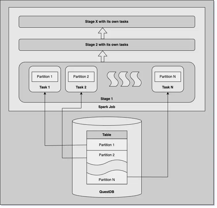
In this tutorial, we will load data from a QuestDB table into a Spark
application and explore the inner working of Spark to refine data loading.
Finally, we will modify and save the data back to QuestDB.
Loading data to Spark
First thing first, we need to load time-series data from QuestDB. I will use an
existing table, `trades`, with just over 1.3 million rows.
It contains bitcoin trades, spanning over 3 days: not exactly a big data
scenario but good enough to experiment.
The table contains the following columns:
| Column Name | Column Type |
| ----------- | ----------- |
| `symbol` | SYMBOL |
| `side` | SYMBOL |
| `price` | DOUBLE |
| `amount` | DOUBLE |
| `timestamp` | TIMESTAMP |
The table is partitioned by day, and the `timestamp` column serves as the
designated timestamp.
QuestDB accepts connections via...
### Processing Time-Series Data with QuestDB and Apache Kafka
**URL**: https://questdb.com/blog/processing-time-series-with-questdb-apache-kafka/
**Description**: Streaming market data to QuestDB using Golang and Apache Kafka
[Apache Kafka](/docs/ingestion/message-brokers/kafka/) is a battle-tested
distributed stream-processing platform popular in the financial industry to
handle mission-critical transactional workloads. Kafka's ability to handle large
volumes of real-time market data makes it a core infrastructure component for
trading, risk management, and fraud detection. Financial institutions use Kafka
to stream data from market data feeds, transaction data, and other external
sources to drive decisions.
A common data pipeline to ingest and store financial data involves publishing
real-time data to Kafka and utilizing Kafka Connect to stream that to databases.
For example, the market data team may continuously update real-time quotes for a
security to Kafka, and the trading team may consume that data to make buy/sell
orders. Processed market data and orders may then be saved to a time series
database for further analysis.
In this article, we'll create a sample data pipeline to illustrate how this
could work in practice. We will poll an external data source (FinnHub) for
real-time quotes of stocks and ETFs, and publish that information to Kafka.
Kafka Connect will then grab those records and publish it to a time series
database (QuestDB) for analysis.
Prerequisites
- Git
- Docker Engine: 20.10+
- [Golang 1.19+](https://go.dev/doc/install)
- [FinnHub API Token](https://finnhub.io/)
Setup
To run the example locally, first clone the
[repo](https://github.com/Yitaek/stocks-kafka-questdb)
The codebase is organized into three parts:
- Golang code is located at the root of the repo
- Dockerfile for the Kafka Connect QuestDB image and the Docker Compose YAML
file is under docker
- JSON files for Kafka Connect sinks are under `kafka-connect-sinks`
Building the Kafka Connect QuestDB Image
We first need to build the Kafka Connect docker image with QuestDB Sink
connector. Navigate to the `docker` directory and run `docker-compose build`.
The Dockerfile is simply installing t...
### The Inner Workings of Distributed Databases
**URL**: https://questdb.com/blog/inner-workings-distributed-databases/
**Description**: Comparison of replication options of time-series databases.
> This post examines the various replication strategies used by popular
> time-series and
> [OLAP databases](/blog/olap-vs-time-series-databases-the-sql-perspective/) to
> implement high-availability. Our learnings from this research have inspired us
> as we continue to build replication into our own performance-focused database,
> [QuestDB](https://github.com/questdb/questdb). The database is built in C++,
> low latency Java, and recently Rust! The codebase has no external dependencies
> and we implement SQL with native time-series extensions.
After being unable to ride my new electric bike to work yet again because it was
in the shop (this time because of a wiring problem that prevented the bike from
running!), I started to think about how I could create some redundancy in my
biking setup so I wouldn't be stuck riding the Tube for weeks at a time due to
simple maintenance or a supply chain issue. What if I had another bike to ride
while my current one is being fixed? That would definitely help, but electric
bikes are expensive, and there's little room to store a backup bike in my cozy
London apartment.
Believe it or not, this problem is similar to what I've been tackling at my day
job as a database developer. Just like bicycles, databases can break down too!
Sometimes hardware fails mysteriously, or a network config has changed and your
database is no longer reachable. Sure, you could always restore your data from a
backup onto new hardware in the event of a failure, but then you're stuck with
downtime and potentially lost data; and that's assuming you've tested your
restore process recently to ensure that it even works! Even if you're able to
run a restore seamlessly, just like I need to wait for the shop to finish fixing
my bike before I can start riding it to work again, you would also need to wait
for the restore to complete and the new database to be configured before using
it.
But luckily, unlike my bike situation, modern databases have the capabi...
### Migrating from Relational Databases to Time-series Databases
**URL**: https://questdb.com/blog/migrating-relational-databases-time-series-databases/
**Description**: The unique characteristics of time-series data and some options to consider when migrating from a relational database to a time-series database.
Learn more about the unique characteristics of time-series data and some options
to consider when migrating from a
[relational database](/glossary/relational-database/) to a
[time-series database](/glossary/time-series-database/).
[Read more](https://itnext.io/migrating-from-relational-databases-to-time-series-databases-9f059a3e34cb)
### MongoDB Time Series Benchmark and Review
**URL**: https://questdb.com/blog/mongodb-time-series-benchmark-review/
**Description**: A comparison between MongoDB and QuestDB focusing on performance and user experience.
This article compares QuestDB with one of the most popular databases on the
market, [MongoDB](https://www.mongodb.com/). We look at the two databases in
terms of benchmark performance and user experience.
```info
These benchmarks predate QWP, the binary protocol we shipped in
[QuestDB 10.0](/blog/questdb-10-release/) in August 2026. Ingestion here runs
over InfluxDB Line Protocol, a text format the server parses row by row. QWP
sends binary columns instead, up to
[3.6x faster over a network](/blog/qwp-vs-ilp-ingestion-benchmark/), and it
[streams reads back as Arrow](/blog/streaming-500-million-rows-into-apache-arrow/).
Read the QuestDB figures below as a floor.
```
Introduction to time-series databases
[Time-series data](/blog/what-is-time-series-data/)has gained popularity in
recent years. It is used in a wide variety of industries and use cases. As a
result, we have seen the emergence of new
[time-series databases](/glossary/time-series-database/), either purposefully
built to handle [time-series data](/blog/what-is-time-series-data/), or as an
additional functionality on top of a general-purpose database. Time series data
is often processed with dedicated tooling. This is because handling this type of
data has a few individual requirements:
- Time series data is often continuously appended (streamed in) from sources
such as market data providers, sensors or via message brokers such as
[Kafka](/docs/ingestion/message-brokers/kafka/).
- The significance of data typically decreases over time. Older data is often
less critical than newer one.
- Recent data often needs to be processed and analyzed quickly, in real-time.
Based on these traits, the evaluation of a
[time-series database](/glossary/time-series-database/) should cover the
following characteristics:
- High ingestion speed to process large amounts of data with
[high cardinality](/glossary/high-cardinality/)
- Fast queries for data analysis "on the fly"
- Ease of use with a well-known l...
### Loading Pandas DataFrames into QuestDB
**URL**: https://questdb.com/blog/loading-pandas-dataframes/
**Description**: Learn how to use the QuestDB Python package to ingest Pandas DataFrames.
```warning
At the time of publishing, this was the recommended way to load pandas
DataFrames into QuestDB. It is now outdated, and the ingestion code below no
longer runs against current clients, which take the protocol as `Sender`'s
first argument. Since QuestDB 10.0 the first-party
[Python client](/docs/connect/clients/python/) covers both directions
natively: `db.dataframe()` ingests a whole frame column by column, and query
results come back with `to_pandas()`. See
[Pandas integration](/docs/integrations/data-processing/pandas/) for the
current approach.
```
Pandas is an open-source data analysis and data manipulation library for Python
that has become an essential tool for data scientists and analysts. It provides
a simple and intuitive way to manipulate data, making it a popular choice for
data analysis tasks. However, while Pandas is excellent for small to
medium-sized datasets, it can struggle with large datasets that exceed the
available memory of the machine it is running on.
This is where QuestDB comes in, as it is well suited for processing large
time-series datasets. By loading Pandas DataFrames into QuestDB, we can leverage
[powerful data processing capabilities](https://github.com/questdb/py-tsbs-benchmark#serialization-network-send--data-insertion-into-questdb)
of the database, allowing you to analyze and manipulate large datasets.
In this tutorial, we will learn how to load large Pandas dataframes into
QuestDB. We use yellow and green taxi trip records published by NYC Taxi &
Limousine Commission as our data source.
Prerequisites to start loading Pandas DataFrames into QuestDB
For this tutorial, it is recommended to have a basic understanding of Python,
and SQL. Also, you will need to have the following installed on your machine:
- Docker
Downloading the dataset before loading it using Pandas
Before we begin loading the data into QuestDB, we need to obtain the data that
we will be working with. As mentioned above, we will use the NYC...
### Running Databases on Kubernetes
**URL**: https://questdb.com/blog/databases-on-k8s/
**Description**: Things to consider when running a database on Kubernetes.
{/* prettier-ignore-start */}
A few weeks ago, [Kelsey Hightower](https://twitter.com/kelseyhightower)
[wrote a tweet](https://twitter.com/kelseyhightower/status/1624081136073994240)
and held a
[live discussion on Twitter](https://twitter.com/kelseyhightower/status/1624096644865327105)
about whether it's a good idea or not to run a database on Kubernetes. This
happened to be incredibly timely for me, since we at QuestDB are about to launch our own cloud database service (built on top of
k8s)!
"Rubbing Kubernetes on Postgres won't turn it into Cloud SQL"
> Tweet from Kelsey Hightower{" "}
via Twitter
> You can run databases on Kubernetes because it's fundamentally the same as
> running a database on a VM. The biggest challenge is understanding that
> rubbing Kubernetes on Postgres won't turn it into Cloud SQL. 🧵
One of the biggest takeaways from this discussion is that there seems to be a
misconception about the features that k8s actually provides. While newcomers to
k8s may expect that it can handle complex application lifecycle features
out-of-the-box, it in fact only provides a set of cloud-native primitives (or
building blocks) for you to configure and use to deploy your workflows. Any
functionality outside of these core building blocks needs to be implemented
somehow in additional orchestration code (usually in the form of an operator) or
config.
K8s Primitives
When working with databases, the obvious concern is data persistence. Earlier in
its history, k8s really shined in the area of orchestrating stateless workloads,
but support for stateful workflows was limited. Eventually, primitives like
[StatefulSets](https://kubernetes.io/docs/concepts/workloads/controllers/statefulset/),
[PersistentVolumes](https://kubernetes.io/docs/concepts/storage/persistent-volumes/)
(PVs), and PersistentVolumeClaims (PVCs) were developed to help orchestrate
stateful workloads on ...
### Unstable CI builds and open-source infrastructure
**URL**: https://questdb.com/blog/maven-troubleshooting-open-source/
**Description**: A story about troubleshooting and fixing an issue in Apache Maven
Donald Knuth [famously wrote](https://dl.acm.org/doi/10.1145/356635.356640) that
Premature Optimization is the root of all evil. I, for one, believe that all
evil comes from spuriously failing builds. Nothing steals my confidence in a
project as quickly as unstable builds alternating between green and red for no
reason. This is a story about unstable builds and troubleshooting. More
importantly, this story is written to thank all contributors to basic software
infrastructure - the infrastructure we all use and take for granted.
Surprise in logs
Upon logging into
[Azure Pipelines](https://azure.microsoft.com/en-gb/products/devops/pipelines/)
to review the logs of multiple failed builds, I mentally braced myself for a
potentially arduous troubleshooting session. I suspected that a race condition
was the culprit that caused non-deterministic outcomes. Therefore, I was
surprised to discover the actual reasons for the recent build failures. They
were all similar to this:
```
2023-02-22T13:57:55.6111290Z [ERROR] Plugin org.apache. Maven.plugins:maven-clean-plugin:3.2.0 or one of its dependencies could not be resolved: Failed to read artifact descriptor for org.apache.maven.plugins:maven-clean-plugin:jar:3.2.0: Could not transfer artifact org.apache.maven.plugins:maven-clean-plugin:pom:3.2.0 from/to central (https://repo.maven.apache.org/maven2): Connection reset -> [Help 1]
2023-02-22T13:57:55.6113250Z [ERROR]
2023-02-22T13:57:55.6126660Z [ERROR] To see the full stack trace of the errors, re-run Maven with the -e switch.
2023-02-22T13:57:55.6127480Z [ERROR] Re-run Maven using the -X switch to enable full debug logging.
2023-02-22T13:57:55.6127880Z [ERROR]
2023-02-22T13:57:55.6128720Z [ERROR] For more information about the errors and possible solutions, please read the following articles:
2023-02-22T13:57:55.6129520Z [ERROR] [Help 1] http://cwiki.apache.org/confluence/display/MAVEN/PluginResolutionException
```
This was the most interesting part:
`Could not tra...
### QuestDB with Python, Pandas, and SQL in a Jupyter notebook
**URL**: https://questdb.com/blog/questdb-demo-python-pandas-sql-jupyter/
**Description**: Interactive Jupyter Lab environment with QuestDB, Python, and time-series energy data.
We built `play` for anyone to try our database in a very easy way. There’s a
Jupyter Lab notebook, data, sample code, queries, and graphs. The data is grid
energy usage and forecasts at 15-minute intervals. You’ll be able to play with
just under half a million rows, try out queries and plot a few graphs.
[Try it out now!](https://play.questdb.io/)
### UUID: Coordination-Free Unique Keys and Why They are Useful
**URL**: https://questdb.com/blog/uuid-coordination-free-unique-keys/
**Description**: Introduction to the UUID data type and coordination-free unique IDs
Let’s build an IoT application with weather sensors deployed around the globe.
The sensors will collect data and we store the data along with the IDs of the
sensors. We’ll run multiple database instances, and the sensors will write to
the geographically closest database. All databases will regularly exchange data,
so eventually, all the databases will have data from all the sensors.
We need each sensor to have a globally unique ID. How can we achieve it? For
example, we could run a service assigning sensor IDs as a part of the sensor
installation procedure. It would mean additional architectural complexity, but
it's doable. Sensor IDs are immutable, so each sensor needs to talk to the ID
service only once - right after the installation. That’s not too bad.
What if we need to store a unique ID for each data reading? Hitting the
centralized ID service whenever we need to store data is not an option. That
would stress the ID service too much and when the ID service is unavailable no
sensor could write any data.
What are the possible solutions?
In the simplest case, each sensor could talk to the remote ID service and
reserve a block of IDs it could then assign locally without further
coordination. When it exhausts the block, it asks the ID service for a new one.
This strategy would reduce the load on the ID service, and sensors could
function even when the ID service is temporarily unavailable. We could also
generate local reading IDs and prefix them with our unique immutable sensor ID.
We could also be smart and use fancy ID algorithms like FlakeIDs.
The strategies mentioned aim to minimize the need for coordination while still
making sure that the IDs are unique globally. The goal is to generate unique IDs
without any coordination at all. This is what we call coordination-free unique
IDs.
UUID enters the scene
Flip a coin 128 times and write down 1 for each head and 0 for each tail. This
gives you a sequence of 128 1s and 0s, or 128 bits of randomness. ...
### Data Integration for Time-Series: ETL, ELT, and CDC
**URL**: https://questdb.com/blog/data-integration-time-series-etl-elt-cdc/
**Description**: An overview of popular data integration strategies with a highlight on CDC.
As digital transformation reaches more industries, the number of data points
generated is growing exponentially. As such, data integration strategies to
collect such large volumes of data from different sources in varying formats and
structures are now a primary concern for data engineering teams. Traditional
approaches to data integration, which have largely focused on curating highly
structured data into data warehouses, struggle to deal with the volume and
heterogeneity of new data sets.
[Time-series data](/blog/what-is-time-series-data/) present an additional layer
of complexity. By nature, the value of each time series data point diminishes
over time as the granularity of the data loses relevance as it gets stale. So it
is crucial for teams to carefully plan data integration strategies into
[time-series databases](/glossary/time-series-database/) (TSDBs) to ensure that
the analysis reflects the [trends](/glossary/time-series-analysis/#trend) and
situation in near real-time.
In this article, we'll examine some of the most popular data integration
solutions for [time-series databases](/glossary/time-series-database/):
- **ETL** (Extract, Transform, Load)
- **ELT** (Extract, Load, Transform)
- **[Data Streaming](/glossary/stream-processing/) with CDC**
[(Change Data Capture)](/glossary/change-data-capture/)
Given the need for real-time insights for time series data, many modern
event-driven architectures now implement data streaming with CDC. To illustrate
how it works in practice, we will walk through a reference implementation with
QuestDB to show that CDC can flexibly handle the needs of a time series data
source.
Extract, Transform, Load (ETL)
ETL is a traditional and popular data integration strategy that involves first
transforming the data into a predetermined structure, before loading the data
into the target system (typically a data warehouse).
One of the main advantages of ETL is that it provides the highest degree of
customization. Sinc...
### EXPLAIN Your SQL Query Plan
**URL**: https://questdb.com/blog/explain-sql-query-plan/
**Description**: Introduction to EXPLAIN command, which can help with performance tuning
We recently implemented the [`EXPLAIN`](/docs/query/sql/explain/) SQL
keyword. In this new series of articles, we are going to shed light on how to
fine tune your SQL queries to improve performance, with the help of `EXPLAIN`.
We start the first post of this series with an introduction to the `EXPLAIN`
execution plan.
Optimization in SQL
One of the first tasks I got when I started working as a Java software developer
was about optimization: optimization for nightly processes of an online
reservation system, a traditional three-tiered Java web application backed by
then-popular RDBMS. A story like many others - processes that started fast and
nimble became slow and resource-hungry over the years, up to a point where they
were running late, overlapped with daily load, or just errored out.
Not good.
Quick code reconnaissance showed that the said batch processes relied heavily on
the database. They ran many custom multi-page-long SQLs one after another and
exported some results to data files. Checking logs revealed that some took
seconds while others dragged on for tens of minutes. Profiling JVM only showed
that the application is waiting on queries. System logs weren't more useful than
that - they showed lots of IO and CPU load but didn't give any hint as to why.
It seems the only option is to speed up queries.
Right, but how?
At first, I had no idea. I simply took the slowest query and started making
changes here and there. Most changes didn't improve the query speed, and when
they did, it turned out that the query was broken. Applying good advice from
Internet forums didn't help at all. After a few hours, I gave up and tried
asking local database gurus for help. To my surprise, the suggestions I received
were repeating the 'Internet wisdom', e.g.:
- "Use hint X."
- "`UNION` is slow, rewrite it to `UNION ALL`."
- "You have to use index, because full table scan is slow."
While still trying to apply any advice I could find and feeling tired, I
discovere...
### Three SQL Keywords for Finding Missing Data
**URL**: https://questdb.com/blog/three-sql-keywords-for-finding-missing-data/
**Description**: How to use QuestDB's SQL keywords to identify gaps in your database
Whether you are just starting to work with a specific data set or monitoring
activities and reports based on existing data sets, one of the first things you
need to consider is the quality of the data you're dealing with. Continuity is
one of the most critical factors in gauging the quality of
[time-series data](/blog/what-is-time-series-data/). Time-series systems usually
serve use cases where data needs to be consumed, processed, and acted upon with
urgency.
Take the example of a public transport vehicle. For the safety of passengers and
the timeliness of the service, vehicles need their various sensors - GPS,
proximity sensors, pressure sensors, engine diagnostics sensors, and so on.
Continuously using the data from these sensors helps the public transport
service guarantee timeliness, safety, and reliability. However, a break in the
data coming from these sensors would mean that there’s a problem.
Most data access frameworks, including query languages and importable libraries,
allow you to filter and see columns or rows where data is missing. The concept
of data continuity and completeness isn't more relevant anywhere than when
you're talking about [time-series data](/blog/what-is-time-series-data/). By
definition, [time-series data](/blog/what-is-time-series-data/) needs to be
continuous. However, the granularity of the continuum might differ for different
requirements.
When you have to test your data for completeness in a
[relational database](/glossary/relational-database/), you often have to write
complex SQL queries paired with intermediate or temporary tables to find missing
data. In some cases, these queries can be tedious and non-performant. QuestDB is
a [time-series database](/glossary/time-series-database/) that lets you store
and consume your data in tabular form, but it's not what you would call a
traditional relational database. To cater to the time-series workloads, QuestDB
extends the standard SQL functionalities using SQL extensions. O...
### Using QuestDB to collect infrastructure metrics
**URL**: https://questdb.com/blog/questdb-cloud-metrics-kubernetes/
**Description**: An article with a hands-on example of how QuestDB is using our own database to monitor our Cloud Platform.
One of my favorite things about QuestDB is the ability to write queries in SQL
against a high-performance time series database. Since I've been using SQL as my
primary query language for basically my entire professional career, it feels
natural for me to interact with data using SQL instead of other newer
proprietary query languages. Combined with QuestDB's
[custom SQL extensions](https://questdb.com/docs/concepts/deep-dive/sql-extensions/), its
built-in SQL support makes writing complex queries a breeze.
In my life as a Cloud Engineer, I deal with time series metrics all the time.
Unfortunately, many of today's popular metrics databases don't support the SQL
query language. As a result, I've become more dependent on pre-built dashboards,
and it takes me longer to write my own queries with JOINs, transformations, and
temporal aggregations.
QuestDB can be a great choice for ingesting application and infrastructure
metrics, it just requires a little more work on the initial setup than the
Kubernetes tooling du jour. Despite this extra upfront time investment (which is
fairly minimal in the grand scheme of things), I think that the benefits of
using QuestDB for infrastructure metrics are worth it. With QuestDB, you get
[industry-leading performance](https://questdb.com/blog/2021/06/16/high-cardinality-time-series-data-performance/)
and the ability to interact with the database in the most commonly-used query
language in existence.
In this article, I will demonstrate how we use QuestDB as the main component in
this new feature. This should provide enough information for you to also use
QuestDB for ingesting, storing, and querying infrastructure metrics in your own
clusters.
Architecture
[Prometheus](https://prometheus.io/) is a common time series database that is
already installed in many Kubernetes clusters. We will be leveraging its
[remote write](https://prometheus.io/docs/practices/remote_write/) functionality
to pipe data into QuestDB for querying and ...
### Realtime crypto tracker with QuestDB Kafka Connector
**URL**: https://questdb.com/blog/realtime-crypto-tracker-with-questdb-kafka-connector/
**Description**: Send real-time cryptocurrency metrics to Kafka topics, ingest to QuestDB, and calculate moving averages with Pandas.
As someone interested in the future of DeFi
([decentralized finance](https://yitaek.medium.com/intro-to-defi-b4ab2ec0f156)),
I wanted to better track the price of different cryptocurrencies and store them
into a timeseries database for further analysis. I found an interesting talk by
Ludvig Sandman and Bruce Zulu at Kafka Summit London 2019,
[Using Kafka Streams to Analyze Live Trading Activity for Crypto Exchanges](https://www.confluent.io/kafka-summit-lon19/using-kafka-streams-analyze-trading-crypto-exchanges/),
so I decided to leverage Kafka and modify it for my own use.
QuestDB is a fast, open-source,
[time-series database](/glossary/time-series-database/) with SQL support. This
makes it a great candidate to store financial market data for further historical
trend analysis and generating trade signals. The team has released an official
[QuestDB Kafka connector](/docs/ingestion/message-brokers/kafka/).
Underneath the hood, the new connector uses InfluxDB line protocol (ILP), which
has excellent ingestion performance and easy schema management. So I decided to
give this a spin and apply it to my project,
[kafka-crypto-questdb](https://github.com/Yitaek/kafka-crypto-questdb).
Prerequisites
- [Docker](https://docs.docker.com/get-docker/) with at least 4GB memory
- [Python 3.7+](https://www.python.org/download/) and
[pip](https://pypi.org/project/pip/)
- [GitHub repository](https://github.com/Yitaek/kafka-crypto-questdb) which
contains the source for the examples below
**Note:** Memory can be increased on Docker Desktop in **Settings -> Resources
-> Memory** and increasing the default limit from `2GB` to `4GB`.
Project setup
At a high level, this project polls the public Coinbase API for the price of
Bitcoin, Ethereum, and Chainlink. This information was then published onto
individual topics on [Kafka](/docs/ingestion/message-brokers/kafka/) (e.g.
topic_BTC) and sent to QuestDb via Kafka Connect:
 paradigm to **ELT** (Extract-Load-Transform) where raw
data is first loaded into a data lake before transformations are applied (e.g.,
aggregations, joins) for further analysis. Traditional ETL pipelines were hard
to maintain and relatively inflexible with changing business needs. As new cloud
technologies promised cheaper storage and better scalability, data pipelines
could move away from pre-built extractions and batch uploads to a more streaming
architecture.
[Change data capture (CDC)](/glossary/change-data-capture/) fits nicely into
this paradigm shift where changes to data from one source can be
[streamed](/glossary/stream-processing/) to other destinations. As the name
implies, CDC tracks changes in data (usually a database) and provides plugins to
act on those changes. For event-driven architectures, CDC is especially useful
as a consistent data delivery mechanism between service boundaries (e.g.,
[Outbox Pattern](https://microservices.io/patterns/data/transactional-outbox.html)).
In a complex microservice environment, CDC helps to simplify data delivery logic
by offloading the burden to the CDC systems.
To illustrate, let's take a reference architecture to stream stock updates from
PostgreSQL into QuestDB. A simple Java Spring App polls stock prices by ticker
symbol and updates the current price to a PostgreSQL database. Then the updates
are detected by [Debezium](https://debezium.io/) (a popular CDC system) and fed
to a [Kafka](/docs/ingestion/message-brokers/kafka/) topic. Finally, the
[Kafka Connect QuestDB connector](/docs/ingestion/message-brokers/kafka/)
listens to that topic and streams changes into QuestDB for analysis.
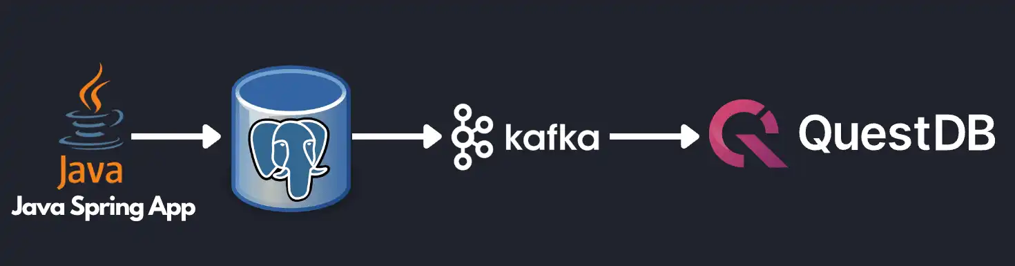
Structuring the data pipeline this way allows the application to be simple. The
Java Spring App only needs to fetch the latest stock data and commit to
P...
### Using Prometheus, Loki, and Grafana to monitor QuestDB in Kubernetes
**URL**: https://questdb.com/blog/2022/12/13/using-prometheus-loki-grafana-monitor-questdb-kubernetes/
**Description**: How to monitor a QuestDB instance using Loki and Prometheus
One of our Cloud engineers, [Steve Sklar](https://github.com/sklarsa), shares
with us how to use some of the most popular tools in the Kubernetes ecosystem to
build monitoring infrastructure for your QuestDB instances.
Monitoring QuestDB in Kubernetes
As any experienced infrastructure operator will tell you, monitoring and
observability tools are critical for supporting production cloud services.
Real-time analytics and logs help to detect anomalies and aid in debugging,
ultimately improving the ability of a team to recover from (and even prevent)
incidents. Since container technologies are drastically changing the
infrastructure world, new tools are constantly emerging to help solve these
problems. Kubernetes and its ecosystem have addressed the need for
infrastructure monitoring with a variety of newly emerging solutions. Thanks to
the orchestration benefits that Kubernetes provides, these tools are easy to
install, maintain, and use.
Luckily, QuestDB is built with these concerns in mind. From the presence of core
database features to the support for orchestration tooling, QuestDB is easy to
deploy on containerized infrastructure. This tutorial will describe how to use
today's most popular open source tooling to monitor your QuestDB instance
running in a Kubernetes cluster.
Components
Our goal is to deploy a QuestDB instance on a Kubernetes cluster while also
connecting it to centralized metrics and logging systems. We will be installing
the following components in our cluster:
- A [QuestDB](https://questdb.com/) database server
- [Prometheus](https://prometheus.io/) to collect and store QuestDB metrics
- [Loki](https://grafana.com/oss/loki/) to store logs from QuestDB
- [Promtail](https://grafana.com/docs/loki/latest/clients/promtail/) to ship
logs to Loki
- [Grafana](https://grafana.com/oss/grafana) to build dashboards with data from
Prometheus and Loki
These components work together as illustrated in the diagram below:
Prerequisites
To foll...
### Listen to Your CPU - Full-table Scans Are Fast
**URL**: https://questdb.com/blog/2022/11/30/full-table-scan-are-fast/
**Description**: Demonstrating the raw speed of modern hardware
One of our core engineers, [Jaromir Hamala](https://x.com/jerrinot), was
inspired by an article comparing performance between index merging and composite
indexes. He conducted a similar test on QuestDB's table scanning strategy. In
this article, Jaromir explains the benefit of table scanning and shows the
superior query performance it brings.
A Hacker News article: index merges and composite indexes
While browsing Hacker News, I stumbled upon an excellent article written by
Simon Hørup Eskildsen:
["Index Merges vs Composite Indexes in Postgres and MySQL"](https://sirupsen.com/index-merges).
Simon compares index performance for queries using a conjunction of two
attributes. This is a fancy way to say that an SQL query contains a predicate
similar to this:
```questdb-sql
WHERE attribute1 = 'foo' AND attribute2 = 'bar;
```
The article does multiple things exceptionally well:
- It describes different strategies a database engine can use to evaluate the
query: composite indexes v.s. merging results from individual indexes.
- It shows systematic thinking about performance. It tries to estimate expected
performance results based on the capabilities of modern hardware in
combination with educated guesses about how a database likely works. I found
this part incredibly fascinating. Reasoning about performance from first
principles is more than just cool. It helps to build a better intuition and
deeper understanding of our tools.
- It shows the actual results from MySQL and PostgreSQL, discusses how they
differ from the expected results, and tries to explain the reasons. Again,
very enlightening!
While reading the article, I wondered: how would QuestDB perform in this
scenario? My curiosity increased after reading a
[discussion](https://news.ycombinator.com/item?id=33765570) on Hacker News -
someone posted results from a similar query running on ClickHouse. So I thought
that it'd be interesting to do a similar one on QuestDB!
To index or not inde...
### QuestDB 6.6.1 - Dynamic Commits
**URL**: https://questdb.com/blog/2022/11/25/questdb-6.6.1-dynamic-commits/
**Description**: The detailed story of how QuestDB 6.6.1 increases data freshness
We are excited to announce the release of
[QuestDB 6.6.1](https://github.com/questdb/questdb/releases/tag/6.6.1), which
brings dynamic commits to optimize ingestion throughput and data freshness for
reads. In this blog post, our CTO, Vlad, shares the story driving the creation
of the dynamic commits.
QuestDB's data structure and out-of-order data ingestion
Many storage systems adopt a Log-Structured Merge tree at their core. QuestDB
differs from them, and the ingested data will always be ordered by timestamp
once it is committed to disk. QuestDB 6.0 enabled out-of-order ingestion,
for which we introduced a commit lag to optimize ingestion throughput for
unordered data. The commit lag includes a time-based buffer and delays the data
commit. This way, out-of-order data can be re-ordered on the fly in memory.
QuestDB's in-memory reordering is particularly efficient, and avoids heavy
copy-on-merge operations, which would be needed otherwise.
As such, we have an implicit trade-off between the ingestion throughput of
unordered data and the availability of data for reads. A higher buffer implies a
longer time delay for the data to be available for reads, while a short buffer
might affect disk write throughput, as we need to reshuffle already committed
out-of-order data.
To recap, when treating the incoming data, the commit lag ensures:
- Data is sorted chronologically.
- New data is merged with the existing one.
- A consistent view of the existing data is maintained for concurrent reads.
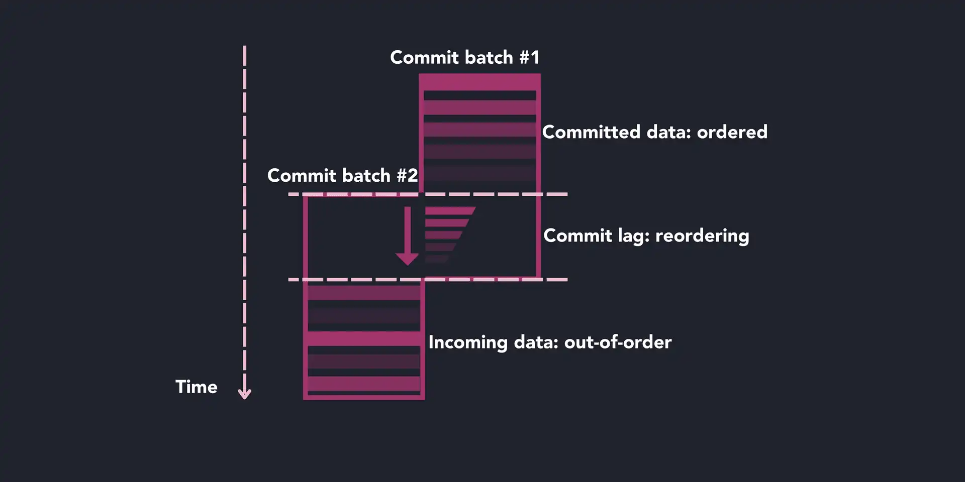
For QuestDB 6.5.5 and earlier versions, users needed to understand the "shape"
of their data to adjust the commit lag value, either through server
configuration or query settings.
A misconfigured commit lag would lead to user pain and frustration: some of our
users would expect data to be available for reads immediately, but the default
configuration was out of whack. For heavy out-of-order ...
### SQL Extensions for Time Series Data in QuestDB - Part II
**URL**: https://questdb.com/blog/2022/11/23/sql-extensions-time-series-data-questdb-part-ii/
**Description**: SQL extensions for time series data in QuestDB part II
This tutorial follows up on our previous one, where we introduced SQL extensions in QuestDB
that make [time series analysis](/glossary/time-series-analysis/) easier. Today,
you will learn about the [`SAMPLE BY` extension](/docs/query/sql/sample-by/)
in detail, which will enable you to work with
[time-series data](/blog/what-is-time-series-data/) efficiently because of its
simplicity and flexibility.
To get started with this tutorial, you should know that `SAMPLE BY` is a SQL
extension in QuestDB that helps you group or bucket
[time-series data](/blog/what-is-time-series-data/) based on the
[designated timestamp](/docs/concepts/designated-timestamp/). This removes the
need for lengthy `CASE WHEN` statements and `GROUP BY` clauses. Not only that,
the `SAMPLE BY` extension enables you to quickly deal with many other
data-related issues, such as
[missing data](/docs/query/sql/sample-by/#fill-options),
[incorrect timezones](/docs/query/sql/sample-by/#time-zone), and
[offsets](/docs/query/sql/sample-by/#with-offset).
This tutorial assumes you have an up-and-running QuestDB instance ready for use.
Let's dive straight into it.
Setup
Import sample data
Similar to the previous tutorial, we'll use
[the NYC taxi rides data for February 2018](https://s3-eu-west-1.amazonaws.com/questdb.io/datasets/grafana_tutorial_dataset.tar.gz).
You can use the following script that utilizes the
[HTTP REST API](/docs/ingestion/import-csv/#import-csv-via-rest/) to upload data
into QuestDB:
```sh
curl https://s3-eu-west-1.amazonaws.com/questdb.io/datasets/grafana_tutorial_dataset.tar.gz > grafana_data.tar.gz
tar -xvf grafana_data.tar.gz
curl -F data=@taxi_trips_feb_2018.csv http://localhost:9000/imp
curl -F data=@weather.csv http://localhost:9000/imp
```
Alternatively, you can use
[the import functionality in the QuestDB console](/docs/getting-started/web-console/overview/#import), as
shown in the image below:
 model, more granular data
(e.g., data collected at second resolution), would yield better results.
However, to train [forecasting](/glossary/forecasting/) models afterwards,
recording data at such high frequency may not be needed and would be costly in
terms of storage and compute.
When I was working for an IoT company, to combat this issue, we stored data in
three separate databases. To show the most up to date value, latest updates were
pushed to a NoSQL realtime database. Simultaneously, all the data was appended
to both a time series database storing up to 3 months of data for quick analysis
and to an
[OLAP database](/blog/olap-vs-time-series-databases-the-sql-perspective/) for
long-term storage. To stop the time series database from exploding in size, we
also ran a nightly job to delete old data. As the size of the data grew
exponentially with IoT devices, this design caused operational issues with
maintaining three different databases.
QuestDB solves this by providing easy ways to
[downsample](/glossary/downsampling/) the data and also detach or drop
partitions when old data is no longer necessary. This helps to keep all the data
in a single database for most operations and move stale data to cheaper storage
in line with a mature data retention policy.
To illustrate, let’s revisit the
[IoT application involving heart rate data](/blog/2021/02/05/streaming-heart-rate-data-with-iot-core-and-questdb/).
Unfortunately, Google decided to
[shut down its Cloud IoT Core service](https://techcrunch.com/2022/08/17/google-cloud-will-shutter-its-iot-core-service-next-year/),
so we’ll use randomized data for this demo.
Populating heart rate data
Let’s begin by running [Qu...
### QuestDB at Big Data LDN 2022
**URL**: https://questdb.com/blog/2022/10/20/questdb-big-data-ldn/
**Description**: Big Data LDN (London) is the UK’s leading free to attend data & analytics conference and exhibition. This year, Javier Ramirez, Developer Advocate at QuestDB, delivered a talk on "Ingesting A Million Time Series Per Second On A Single Instance".
Big Data LDN (London) is UK’s leading data and analytics conference and
exhibition. This year, [Javier Ramirez](https://github.com/javier), Developer
Advocate at QuestDB, delivered a talk on "Ingesting A Million Time Series Per
Second On A Single Instance".
Big Data LDN is the largest event focusing on data in the UK, with two days of
talks in parallel tracks, plus dozens of vendors. This was a great opportunity
to learn about the latest trends and engage with data-minded folks. We asked
Javier to tell us more about the experience.
What was the crowd like?
A good mix of data engineers, data analysts, decision makers, data vendors, and
some students. There were some well-known developer tools and databases, such as
Confluent ([Kafka](/docs/ingestion/message-brokers/kafka/)),
[OLAP database](/blog/olap-vs-time-series-databases-the-sql-perspective/)
ClickHouse, InfluxData (the parent company of InfluxDB), MongoDB, and Fivetran,
to name a few.
Who did you meet?
We actually met a few QuestDB users, which was an absolute pleasure. We also met
a lot of companies with interesting near real time challenges looking for
solutions, and we found some time to talk to other vendors, explore
collaborations, or simply have a friendly talk about QuestDB's data analytics
capacities. Users were from many different backgrounds: companies managing
wireless networks producing thousands of events per millisecond, hedge funds
overseeing a wide variety of assets, and cryptocurrency exchanges. We even had a
great time speaking with a F1 team looking for a time series database. We hope
to see them all soon in our community slack channel!
What did you talk about?
Mostly about fast and big data, but also quite a bit about the internals of
QuestDB and what makes us stand out from the rest. In particular, our latest
developments on optimizing imports using `io_uring`, or the fact that we use
JAVA with near zero Garbage Collection were popular topics. But we mostly talked
about real use case...
### DevStories #1: Time-series for sports prediction markets
**URL**: https://questdb.com/blog/2022/10/03/athletex-interview/
**Description**: This is a brand-new series for which we interviewed different developers in our community. For the post of this series, we interviewed Kevin Kamto, Co-founder at AthleteX.
_DevStories is our brand-new series. We interview developers in our community to
understand how they build applications with QuestDB. For the first post of this
series, we are thrilled to interview
[Kevin Kamto](https://www.linkedin.com/in/kevin-kamto/), Co-founder at
AthleteX._
Hi Kevin, could you tell us more about yourself?
My name is Kevin Kamto. I'm one of the core contributors and co-founders of
AthleteX. That means that on a day to day basis, I operate as the head of sales
and point of coordination for the team.
How did you get to know time series databases in the first place?
I've been working in the IoT space as a developer for many years. For a cool
project I worked on, we needed to create a device that measured the WiFi usage
in the company to observe the day to day patterns. That's when I got introduced
to InfluxDB, one of the time series database pioneers at that time.
Tell us more about AthleteX, what is this project about?
This is the backstory: during the middle of COVID-19, there were a lot of
markets seeing red. So we asked ourselves, what is an investor to do during this
time? As someone who loves sports like soccer and basketball, I thought that if
I could put my money towards an athlete, I could keep it safe.
> This blog post is not investment advice. 😇
The idea of AthleteX is that you can invest in the performance of your favorite
athletes. Essentially, we created a fantasy sports prediction market. You can go
to the platform to either long or short the performance of an athlete by trading
the Athlete Performance Tokens (APTs). The price of an APT is based on an
athlete's in-game statistics. Taking baseball as an example, we determine price
using the Wins Above Replacement (WAR) formula, and the price is updated in
real-time.
How is the use case related to time series databases?
Using MLB (baseball) as an example, some in-game metrics such as bats and home
runs are generated every minute or every five minutes. We must store all that
...
### Join Hacktoberfest 2022 and contribute to QuestDB!
**URL**: https://questdb.com/blog/2022/09/30/hacktoberfest-questdb/
**Description**: Hacktoberfest 2022 is starting! We are super excited to meet with other open source contributors and maintainers. To celebrate this, we put together some hints for you to get started.
Hacktoberfest 2022 is starting soon! We're super excited about joining
Hacktoberfest again and meeting new or returning open-source contributors! 🤝
Hacktoberfest
For those who aren't familiar with Hacktoberfest, it's a month-long online
celebration for open-source softwares and communities. The first 40,000
participants who
[successfully completed the requirements](https://hacktoberfest.com/participation/#contributors)
will be rewarded with a special-edition Hacktoberfest T-shirt 👕 or a tree
planted in your name. 🌴
Participating in Hacktoberfest is one of our approaches to raise awareness and
encourage more developers or technical writers to contribute to open source. We
welcome both code and non-code contributions, such as docs improvement,
tutorials, and blog posts.
⛳ About us
[QuestDB](https://github.com/questdb/questdb) is a high-performance open-source
database for time series. The project is built from scratch in Java and C++ with
no dependencies and zero garbage collection. It is optimized for high-throughput
ingestion over InfluxDB line protocol and fast SQL queries. QuestDB is also one
of the most popular time series databases according to the independent reviewer
[DBEngines](https://db-engines.com/en/ranking/time+series+dbms).
Developers can use QuestDB as a library for java applications.
[Official clients](/docs/ingestion/overview/#first-party-clients) for
[Python](https://github.com/questdb/py-questdb-client),
[Go](https://github.com/questdb/go-questdb-client),
[C, C++, Rust](https://github.com/questdb/c-questdb-client),
[Node.js](https://github.com/questdb/nodejs-questdb-client) and
[.NET](https://github.com/questdb/net-questdb-client) are also available for the
wider developer community.
This year, there are three QuestDB open source projects opted in for
Hacktoberfest:
1. [**QuestDB**](https://github.com/questdb/questdb): QuestDB core database,
mainly written in Java and C++. Check
[CONTRIBUTING.md](https://github.com/questdb/questdb/...
### Importing 300k rows/sec with io_uring
**URL**: https://questdb.com/blog/2022/09/12/importing-300k-rows-with-io-uring/
**Description**: QuestDB 6.5 introduces a new `COPY` commands allowing importing large CSV files. This article reveals the story behind it and highlights the exciting benchmark results using this new SQL command.
In this blog post, QuestDB’s very own
[Andrei Pechkurov](https://github.com/puzpuzpuz) presents how to ingest large
CSV files a lot more efficiently using the SQL
[`COPY`](https://questdb.com/docs/query/sql/copy/) statement, and takes us
through the journey of benchmarking. Andrei also shares insights about how the
new improvement is made possible by `io_uring` and compares QuestDB's import
versus several well-known OLAP and
[time-series databases](/glossary/time-series-database/) in Clickhouse's
ClickBench benchmark.
Introduction
As an open source time series database company, we understand that getting your
existing data into the database in a fast and convenient manner is as important
as being able to ingest and
[query](https://questdb.com/blog/2022/05/26/query-benchmark-questdb-versus-clickhouse-timescale/)
your data efficiently later on. That's why we decided to dedicate our new
release, QuestDB 6.5, to the new parallel
[CSV file import](https://questdb.com/docs/ingestion/import-csv/) feature. In
this blog post, we discuss what parallel import means for our users and how it's
implemented internally. As a bonus, we also share how recent ClickHouse team's
benchmark helped us to improve both QuestDB and its demonstrated results.
How ClickBench helped us improve
Recently ClickHouse conducted a
[benchmark](https://github.com/ClickHouse/ClickBench) for their own database and
many others, including QuestDB. The benchmark included data import as the first
step. Since we were in the process of building a faster import, this benchmark
provided us with nice test data and baseline results. So, what have we achieved?
Let's find out. The benchmark was using QuestDB's HTTP
[import endpoint](https://questdb.com/docs/query/rest-api/#imp---import-data)
to ingest the data into an existing non-partitioned table. You may wonder why it
doesn't use a [partitioned](https://questdb.com/docs/concepts/partitions/) table,
which stores the data sorted by the timestamp values and provid...
### Setting up Basic Authentication for QuestDB open source using Nginx
**URL**: https://questdb.com/blog/2022/08/05/setting-basic-auth-nginx/
**Description**: How to implement Nginx Basic Authentication for QuestDB open source.
This post comes from
Kovid Rathee,
who has put together a tutorial to show how to add extra security by
implementing Nginx Basic Authentication for QuestDB open source.
Introduction
```warning
This article is now obsolete. Starting from [QuestDB 8.0.3](https://github.com/questdb/questdb/releases/tag/8.0.3), you can configure Basic Auth [directly
on QuestDB](https://questdb.com/docs/configuration/overview/#http-server) by setting the `http.user` and `http.password`
parameters.
```
---
Data privacy and security is one of the most critical areas of concern when
working with any data. This is even more true for
[time-series database](/glossary/time-series-database/) because a lot of
[time-series data](/blog/what-is-time-series-data/) deals with highly essential
financial, geospatial, and medical data, among many others.
While QuestDB open source has already
[added authentication on top of the InfluxDB line protocol](/docs/ingestion/ilp/overview/#authentication)
to secure your [time-series data](/blog/what-is-time-series-data/) ingestion
workloads into QuestDB, you might need more layers of security, mainly to
prevent unauthorized access to your critical data from your QuestDB
[Web Console](/docs/getting-started/web-console/overview/).
There are several ways to achieve this, such as
[SSH tunneling](https://en.wikipedia.org/wiki/Tunneling_protocol),
[OAuth](https://oauth.net/),
[token-based auth](https://www.okta.com/au/identity-101/what-is-token-based-authentication/),
etc. However, this article will take you through the most straightforward
authentication setup of them so that you can get started with basic
authentication with minimal effort using Nginx.
```tip
While you can set up authentication for QuestDB open source,
[QuestDB Enterprise](/enterprise/) offers built-in authentication that offers a
hassle-free, Out-of-the-Box solution.
```
How Basic Authentication Works in Nginx
Nginx is a multi-purpose application that can be used as a
[reverse pro...
### Time Series Forecasting with TensorFlow and QuestDB
**URL**: https://questdb.com/blog/2022/06/20/forecasting-with-questdb-and-tensorflow/
**Description**: Timeseries is a type of data used to train machine learning models. You may have numerical data for predicting housing prices or classification data for categorizing dog and cat breeds. It's also the special type of data used for training machine learning algorithms where time is the crucial component.
This post is contributed by
[Gourav Singh Bais](https://www.linkedin.com/in/gourav-singh-bais/), who has
written an excellent tutorial that shows how to build an application that uses
time series data to forecast trends and events using Tensorflow and QuestDB.
Thanks for the submission!
Machine Learning for Timeseries Forecasting
Machine learning is taking the world by storm, performing many tasks with
human-like accuracy. In the medical field, there are now smart assistants that
can check your health over time. In finance, there are tools that can predict
the return on your investment with a reasonable degree of accuracy. In online
marketing, there are product recommenders that suggest specific products and
brands based on your purchase history.
In each of these fields, a different type of data can be used to train machine
learning models. Among them, _time series data_ is used for training machine
learning algorithms where time is the crucial component.
Time series data is complex and involves time-dependent features that go beyond
the scope of what traditional machine learning algorithms like Regression,
Classification, and Clustering are useful for. Thankfully, there are machine
learning models we can use for
**[time series forecasting](/glossary/forecasting/)**.
Predictions resulted from time series forecasting may not be wholly precise due
to the variable nature of time, but they do provide reasonable approximations
that are applicable in a variety of fields. Let’s consider a few use cases:
- **Predictive maintenance:** nowadays, IoT (internet of things), AI (artificial
intelligence), and integrated systems are being embedded into electronic,
mechanical, and other types of devices to make them smart. These IoT devices
have sensors to keep track of relevant values over time; and artificial
intelligence, of which time series forecasting is a component, is used to
analyze this data and make predictions regarding the approximate time at whi...
### 4Bn rows/sec query benchmark: Clickhouse vs QuestDB vs Timescale
**URL**: https://questdb.com/blog/2022/05/26/query-benchmark-questdb-versus-clickhouse-timescale/
**Description**: QuestDB 6.3 brings parallel filter execution optimization to our SQL engine allowing us to reduce both cold and hot query execution times quite dramatically.
> **Update (2025):** This article was written in 2022 using older software versions (QuestDB 6.3.1, ClickHouse 22.4, TimescaleDB 2.6). For up-to-date benchmarks with current versions, see our latest comparisons:
> - [TimescaleDB vs. QuestDB](/blog/timescaledb-vs-questdb-comparison/)
> - [InfluxDB v1/v2 vs. QuestDB](/blog/influxdb-vs-questdb-comparison/)
> - [InfluxDB 3 Core vs. QuestDB](/blog/influxdb3-core-benchmarks/)
QuestDB 6.2, our previous minor version release,
[introduced](https://questdb.com/blog/2022/01/12/jit-sql-compiler/) JIT
(Just-in-Time) compiler for SQL filters. As we mentioned last time, the next
step would be to parallelize the query execution when suitable to improve the
execution time even further and that's what we're going to discuss and benchmark
today. QuestDB 6.3 enables JIT compiled filters by default and, what's even more
noticeable, includes parallel SQL filter execution optimization allowing us to
reduce both cold and hot query execution times quite dramatically.
Prior to diving into the implementation details and running some before/after
benchmarks for QuestDB, we'll be having a friendly competition with two popular
time series and analytical databases, TimescaleDB and ClickHouse. The purpose of
the competition is nothing more but an attempt to understand whether our
parallel filter execution is worth the hassle or not.
Comparing with other databases
Our test box is a c5a.12xlarge AWS VM running Ubuntu Server 20.04 64-bit. In
practice, this means 48 vCPU and 96 GB RAM. The attached storage is a 1 TB gp3
volume configured for 1,000 MB/s throughput and 16,000 IOPS. Apart from that,
we'll be using QuestDB 6.3.1 with the default settings which means both parallel
filter execution and JIT compilation being enabled.
In order to make the benchmark easily reproducible, we're going to use
[TSBS](https://github.com/timescale/tsbs) benchmark utilities to generate the
data. We'll be using so-called IoT use case:
```bash
./tsbs_generate_data...
### Enabling Machine Learning in QuestDB with MindsDB
**URL**: https://questdb.com/blog/2022/04/18/enabling-machine-learning-in-questdb-with-mindsdb/
**Description**: Combine MindsDB and QuestDB for machine learning predictions with SQL.
Combining both MindsDB and QuestDB gives you unbound prediction ability with
SQL.
[Read more](https://mindsdb.com/blog/tutorial-enabling-machine-learning-in-questdb-with-mindsdb/)
### Demo of live crypto data streamed with QuestDB and Grafana
**URL**: https://questdb.com/blog/2022/04/12/demo-live-crypto-data-streamed-with-questdb-and-grafana/
**Description**: Demo of live crypto data streamed with QuestDB and Grafana
At QuestDB we are all about performance. To showcase querying capabilities of
the database we have been running a live demo of historical taxi rides in NYC
with 1.6 billion rows [1] and a geospatial dataset that contains the
locations of 250k unique ships [2] moving over time. You can analyze
this dataset with SQL on our [live instance](https://demo.questdb.io/) and see
how fast each query is processed. Today, we introduce a new dataset on the same
demo instance: crypto market data ingested in real-time from the Coinbase
Exchange. For ingestion, we use a convenient Python library
[Cryptofeed](https://github.com/bmoscon/cryptofeed), a cryptocurrency exchange
feed handler that supports QuestDB. And for visualization, we use
[Grafana](/docs/integrations/visualization/grafana/) to create interactive live charts,
which refresh every 5 seconds.
We ingest the following columns into QuestDB in real-time for each BTC-USDT and
ETH-USDT trades coming through the Coinbase Exchange:
- price
- side (buy/sell)
- amount
- timestamp
To get you started, we added a set of example queries in the live demo of
QuestDB [Web Console](/docs/getting-started/web-console/overview/). These pre-written queries leverage
the standard SQL syntax and time-series SQL extensions in QuestDB. When clicking
on a query, it's automatically added to the SQL editor. Then, click the
Run button or press F9 to execute the query. Despite the
large amount of data stored on the demo instance, the queries should come back
in milliseconds!
Let's go through these sample queries one by one.
Last prices of BTC and ETH
To find out the latest prices of BTC and ETH in USD. We use the
[`LATEST ON`](/docs/query/sql/latest-on/) syntax, which is
native to QuestDB's SQL Engine:
```questdb-sql title="Latest BTC and ETH prices" demo
SELECT * FROM trades
WHERE symbol in ('BTC-USDT', 'ETH-USDT')
LATEST ON timestamp PARTITION BY symbol;
```
Below is a real-time chart for ...
### Crypto Volume Profiles with QuestDB and Julia
**URL**: https://questdb.com/blog/2022/03/29/crypto-volumes-julia-questdb/
**Description**: Build Bitcoin volume curves using Julia and QuestDB to better understand the flow of trading throughout the day.
When is the Bitcoin market most active and how does this activity change
throughout the day? This is an important question to answer for any algorithmic
trading strategy as it is more expensive to trade in low volume (illiquid) times
and this could end up costing you money. In this post, I'll use QuestDB and
Julia to calculate the average intraday volume profile which will show us how
the pattern of trading varies throughout the day.
Environment
I'm using QuestDB version 6.2 and Julia version 1.7. I've installed the
following packages from the Julia general repository.
```julia
using LibPQ
using DataFrames, DataFramesMeta
using PlotThemes
using Plots
using Dates
```
For more information about getting setup with QuestDB read their
[get started with QuestDB](https://questdb.com/docs/deployment/docker/) guide.
Contents
- [Importing CSV's into QuestDB](#importing-csvs-into-questdb-via-julia)
- [Bitcoin daily volume trends](#bitcoin-daily-volume-trends)
- [Bitcoin intraday volume profiles](#bitcoin-intraday-volume-profiles)
- [Smoothing the volume profiles with LOESS](#smoothing-the-volume-profiles-with-loess)
Importing CSVs into QuestDB via Julia
I've written before about connecting a data source to QuestDB in real-time and
[building you own crypto trade database](https://dm13450.github.io/2021/08/05/questdb-part-1.html).
Now I will take a different approach and show you how to use QuestDB with csv
files. This involves connecting to QuestDB using the REST API and passing the
file with a corresponding database schema.
As most of us have our data in CSVs, (despite the flaws) this will hopefully
help you build Bitcoin volume curves using Julia and QuestDB to better
understand the flow of trading throughout the day. ove to a more practical
database solution. I spent most of my Ph.D. wrestling with flat files and could
have saved some time by moving to a database sooner.
In my case, I have a folder of CSV files of BTCUSD trades downloaded from Alpaca
Market...
### Crypto Data Visualization Dashboards with Grafana
**URL**: https://questdb.com/blog/crypto-data-visualization-dashboards-grafana/
**Description**: Learn how to using Python to fetch cryptocurrency data from Coinbase, store it in QuestDB, and visualize the data using Grafana.
This post comes from Tancrede Collard, who has written an excellent tutorial
that shows how to use Python to fetch cryptocurrency data from Coinbase, store
it in QuestDB, and visualize the data using
[Grafana](/docs/integrations/visualization/grafana/). Thanks for the submission,
Tancrede!
Visualizing time series data
When analyzing streaming data such as cryptocurrency or market metrics, the
foundation of the data processing pipeline is efficient storage and queries. To
use this data for insights and analytics, data visualization is a convenient way
to plot and convey [trends](/glossary/time-series-analysis/#trend), create
actionable reports, or even set up alerting.
Most cryptocurrency trading projects will focus on price charts and standard
indicators like [RSI](https://www.investopedia.com/terms/r/rsi.asp) or moving
averages. Derivatives are often overlooked in many cryptocurrency analytics and
visualization projects, and there's plenty to explore, such as the underlying
pricing metrics such as volatility and funding rates.
A lot of common off-the-shelf tools can plot prices over time, but few are
available for derivative features. Having control of the underlying database,
creating custom metrics, and building dashboards based on these metrics allows
us to build our own solutions with custom pricing inputs and models for
derivatives.
In this tutorial, you'll learn how to fetch data from the Coinbase API using a
Python script, load the data into QuestDB and run SQL queries via QuestDB for
derivatives insights. We'll be visualizing data using Grafana so that we can
build dashboards for reporting or alerts based on metrics you care about.
Prerequisites
To follow with this tutorial, you'll need the following:
- [Coinbase](https://www.coinbase.com/signup) account with an
[API key](https://docs.cdp.coinbase.com/coinbase-app/docs/welcome)
- [Homebrew](https://brew.sh/) for macOS users
Installing QuestDB using homebrew
Before we can start storing da...
### How to generate time-series data in QuestDB
**URL**: https://questdb.com/blog/2022/03/14/mock-sql-timeseries-data-questdb/
**Description**: Learn how to mock timeseries data using built-in SQL functions in QuestDB to generate dummy data for testing and rapid prototyping according to your schemas.
This post comes from Gábor Boros, who has written an excellent tutorial that
shows how to mock timeseries data using built-in SQL functions in QuestDB to
generate dummy data for testing and rapid prototyping according to custom
schemas. Thanks for the submission, Gábor!
Mocking and generating time series data
As developers, we often have to generate sample data for numerous reasons:
feeding integration tests, realistic staging environments or developing an
application locally.
This process can be time-consuming, especially when we need data on a bigger
scale. Fortunately, some databases are helping our work and trying to offload
some weight from our shoulders by providing functions to generate data.
This tutorial will cover how to generate test data using QuestDB using built-in
generators so you can quickly mock data similar to your own production data.
Types of time series data
Before diving deep into generating data using QuestDB, we need to take one step
back to discuss what types of time series data we can generate, what "mock data"
is, and what generator functions are available for use. Let's start with the
different types of time series data. We can classify the data based on the
frequency we receive them into two categories: regular and irregular data.
Regular data is received per a pre-defined period, usually collected by a
collector node or sent by an agent. Collecting metrics from a server fits into
this category perfectly, as shown in the tutorial where we
[connected Telegraf with QuestDB](/blog/2021/07/09/telegraf-and-questdb-for-storing-metrics-in-a-timeseries-database/).
The Telegraf agent running on the server collects the metrics on a pre-defined
basis and sends them to the QuestDB instance.
The opposite of regular data is the irregular data which is collected
dynamically. The main point about irregular data is that we cannot predict how
often the data will arrive. As of examples,
[automating ETL jobs](/blog/2021/03/31/automating-etl-jobs-on-...
### Calling on our community members to help us support Ukraine
**URL**: https://questdb.com/blog/2022/03/07/calling-on-our-community-members/
**Description**: We thank all our stakeholders, users and community members for your support during these challenging times.
There is a lot of Ukraine in QuestDB: Our co-founder Vlad and two of our
engineers, Alex and Eugene, are both Ukrainians. This is our response and our
call on all our users to join us in helping the people of Ukraine.
Eugene was working from his home in Kyiv - the war now forced him and his family
to hide in a bunker. Last Thursday he managed to join our daily standup call in
between bombardments and we were glad to see him alive and well. Our collective
prayers go to him and his family.
We deplore the situation and are focussed on supporting our employees. With the
help of other communities we are evaluating the best options for our employees
and their families, offering logistical support and providing the latest
security updates.
We also call on all our users to join us in helping the people of Ukraine -
together, we can make an impact.
- The following [website](https://supportukrainenow.org/) is a source of
information to help people in need through donations and other means.
We thank all our stakeholders, users and community members for your support
during these challenging times.
We hope that peace gets restored in the region quickly.
QuestDB team
### Order Flow Imbalance - A High Frequency Trading Signal
**URL**: https://questdb.com/blog/2022/02/02/order-flow-imbalance/
**Description**: Calculate order flow imbalance and build high-frequency trading signals with QuestDB.
```info
For a hands-on SQL implementation of OFI using QuestDB, see the
[Order Flow Imbalance cookbook recipe](/docs/cookbook/sql/finance/order-flow-imbalance/).
```
Calculate the order flow imbalance and build a high-frequency trading signal
with the results.
[Read more](https://dm13450.github.io/2022/02/02/Order-Flow-Imbalance.html)
### QuestDB 6.2 January release, SQL JIT compiler
**URL**: https://questdb.com/blog/2022/01/27/release-sql-jit-compiler/
**Description**: We've released version 6.2 and here are the highlights including SQL JIT compiler, JDK 17 support, SQL and ILP improvements and autocomplete in the Web Console.
We've just published 6.2 and it includes a lot of changes, such as SQL JIT
compiler, JDK 17 support, SQL and ILP improvements, settings to improve the
memory footprint when used with [Grafana](/docs/integrations/visualization/grafana/),
autocomplete in the [Web Console](/docs/getting-started/web-console/overview/), improved ILP stability,
and more. Here's a roundup of changes that have just landed in the latest and
greatest version!
JDK 17 support
QuestDB is now compatible with JDK 17, the latest long-term support (LTS) Java
release. We also updated the binary distributions and the Docker image to use
OpenJDK 17.
Just-in-Time compiler for SQL engine
Release 6.2 brings a brand new JIT (Just-in-Time) compiler as a part of the SQL
engine. The compiler aims to significantly improve execution times for queries
with simple arithmetic expressions used to filter the data.
To give you an impression on the performance improvements, let's consider the
following query on the `trips` table that we use in our
[live demo](https://demo.questdb.io/):
```sql
SELECT count(), max(total_amount), avg(total_amount)
FROM trips
WHERE total_amount > 150 AND passenger_count = 1;
```
The below image shows the execution time for this query with and without enabled
[JIT compiler](/docs/concepts/deep-dive/jit-compiler/):
The SQL JIT compiler is a beta feature and is disabled by default. To enable it,
you should change the `cairo.sql.jit.mode` setting in your `server.conf` file.
```ini title="path/to/server.conf"
cairo.sql.jit.mode=on
```
When QuestDB starts with the enabled JIT compiler, the server logs contain
messages relating to `SQL JIT compiler` like the following:
```log
2021-12-16T09:25:34.472450Z A server-main SQL JIT compiler mode: on
2021-12-16T09:25:34.472475Z A server-main Note: JIT compiler mode is a beta feature.
```
JIT compilation won't take place for any query you run. To learn when the
compilation took place for a query, you should check the server logs to co...
### How we built a SIMD JIT compiler for SQL in QuestDB
**URL**: https://questdb.com/blog/2022/01/12/jit-sql-compiler/
**Description**: QuestDB 6.2.0 brings a brand new JIT (Just-in-Time) compiler as a part of the SQL engine. This post describes our storage model, how we built a JIT compiler for SQL and our plans for improving it in future.
QuestDB 6.2.0 brings a brand new JIT (Just-in-Time) compiler as a part of the
SQL engine. The compiler aims to significantly improve execution times for
queries with simple arithmetic expressions used to filter the data. It took us
11K lines of code, 250+ commits, and plenty of coffee to ship it, and we'd like
to share the story with you.
Before we dive into the implementation details behind our
[JIT compiler](/docs/concepts/deep-dive/jit-compiler/), let's understand what kind of
problems JIT compilation aims to solve in our SQL engine and where exactly you
should expect performance improvements.
It can often happen that analytical queries run by users end up performing a
full scan over a table or, at least, over some of its partitions. Here is an
example of such a query:
```questdb-sql
SELECT *
FROM trips
WHERE pickup_datetime IN ('2009-01') AND total_amount > 150;
```
The above query returns relatively expensive trips within one month from 10+
years of taxi data available on our [live demo](https://demo.questdb.io/). To
execute this query, QuestDB has to scan 13.5 million rows. This means that the
database has to do many sequential reads from the column files and apply the
filter expression (think, `WHERE` clause) to each value. There is a good chance
that the data is already in the page cache or the disk is fast enough not to
become the bottleneck. Thus, the execution time for such queries has all chances
to be limited by the CPU performance.
The pre-JIT implementation of filter expression evaluation in QuestDB is based
on the operator function call tree. The functions are nothing more than Java
classes you may find
[as part of the Griffin engine](https://github.com/questdb/questdb/tree/master/core/src/main/java/io/questdb/griffin/engine/functions).
This approach is quite powerful and general, but it also has some disadvantages
we will cover.
Pre-JIT filtering
As you may already know, QuestDB has a
[column-based storage model](/docs/architecture/qu...
### Our two-year journey to raise $15m in venture capital
**URL**: https://questdb.com/blog/2022/01/03/two-year-journey-raising-15m-venture-capital/
**Description**: We've raised over $15 million in venture capital to fund development of the fastest open source time series database. This post describes our two-year journey to raising our $12.5m Series A, what we learned along the way, and the pitch deck we used.
Since founding QuestDB, we've raised over $15 million in venture capital to fund
the development of the fastest open source time series database. This blog post
describes the two-year journey to raise our Series A, what we learned along the
way and the pitch deck we used for the raise.
Founding an open-source company
I met my co-founder Vlad at a fintech startup and he told me about a project of
his that was 5 years in the making. "I have built a database from scratch and I
want to make it open source to empower developers to store large amounts of data
efficiently. It's a fast database that doesn't use code dependencies and you can
access the data with SQL". We discussed the ins and outs of why people need a
system like this and I was all-in on the idea of starting a company around it.
We started our journey in London, which hadn't typically been the birthplace of
successful open source databases. Pitching a database made from scratch with an
optimized codebase in zero-GC Java/C++ to squeeze every bit of performance from
modern hardware wasn't an easy affair. Most of the venture capital funds we
initially met were struggling to understand the value proposition, especially
for an open-source product that wasn't generating revenue at the time.
Preparing for a seed round
In the spring of 2020 we were asking for $2m to hire a few talented engineers
and work on the product. We eventually met a few VCs who saw the potential from
a technological standpoint but wanted to see revenue even though we incorporated
the company a few weeks before. We then met a believer, Paul at the VC firm
Episode 1, who had lived in the bay area for decades. He understood the
potential of open source and community building to fuel developer adoption. We
eventually convinced several other European funds with a growing interest in
open source startups such as Seedcamp to invest as well. In March 2020, we
raised $2m overall, which kicked things off.
We launched an open source versio...
### Analyzing Financial Time-Series Data via the Julia Language and QuestDB
**URL**: https://questdb.com/blog/analyzing-financial-time-series-data-julia-language-questdb/
**Description**: Dean Markwick explores high-frequency finance in Julia and QuestDB: trade prices, returns, autocorrelation, and empirical price impact on crypto data.
What's the difference between finance and high-frequency finance?
I like to think of this question as taking a microscope to finance data and
magnifying everything up to see the nitty-gritty. Most people start by
downloading daily stock prices from something like Yahoo or Google finance. For
some applications, this type of data is enough if you are looking at long-term
trends or say differences between countries, but a whole other world is lurking
underneath those four daily prices.
In the not-so-distant past, getting your hands on more granular data was either
expensive or out of reach to the hobbyist, but there has since been a revolution
thanks to crypto. Now, many crypto exchanges provide their data for free and
this combined with some excellent open-source (and free) tools allow you to
build your own little high-frequency research labs.
This tutorial will hold your hand and introduce you to the concepts of
high-frequency finance and what makes it different. If you are finance-curious
this is the tutorial for you and with Julia and QuestDB I will highlight some of
the basic concepts behind modern data-driven finance.
This tutorial is broken down into the following sections:
1. **The dataset:** what kind of data are we working with?
2. **Prices:** what does a high-frequency price source look like?
3. **Returns:** how do we prepare the data for analysis and how are the returns
distributed?
4. **Correlations:** what does the correlation look like between returns?
5. **Trades:** how can we measure price impact using high-frequency trades?
Creating a dataset of crypto trades from Coinbase
I've written about hooking up to the Coinbase API and storing the results in
QuestDB. It's a technical post and you can
[read the tutorial here](/blog/2021/09/17/high-frequency-finance-julia-lang/).
By using the same process as highlighted in that post, I have stored Bitcoin-USD
exchange rate data and trade data from 09:00 on the 24th of July 2021 to 14:30
on the 2...
### Why I joined QuestDB as a core database engineer
**URL**: https://questdb.com/blog/2021/11/09/miguel-arregui-working-at-questdb/
**Description**: The story of how Miguel Arregui joined as a software engineer building the fastest open source time series database.
This post was written by Miguel Arregui, who describes how he developed a
passion for computing early on, his experience in research at CERN and the ESA,
and eventually working at QuestDB. Miguel works as a software engineer in the
core database team, improving upon the internals of the fastest open source time
series database.
My introduction to computing
My parents are the kind that pursues crafty hobbies after work and involves
their children, so my childhood was great. I came into existence at
`1978-02-28T08:00:00.000000Z`. We helped our mechanical engineer dad in the
garage and our tailoress mom in her studio. It became ingrained in us to never
waste time. When we finished school, I would either do crafty stuff at home or
do something else, most competitive sports like sailing and tae-kwon-do.
One day on `1989-05-11T09:00:00.000000Z`, I received a gift of an
[Amstrad CPC 464](https://en.wikipedia.org/wiki/Amstrad_CPC_464) with a matching
green phosphorous screen. This was my first encounter with computing. I played
many games, learned to copy them (tapes) for sharing, invited friends to code
some basic, or transcribe code examples from coding books. Back then, owning a
computer was the exception and a sure flag for nerdiness that I happily wore.
My second encounter with computing took place in the form of an Intel Pentium my
dad bought "for work." The whole family shared an email account and would warn
each other not to pick up the phone. The internet connection was set up over the
same twisted copper wire that also served the phone. I learned DOS and Pascal,
later some Linux booted from a floppy, and I was hooked. A little later, I
started my university years, entirely devoted to learning the discipline,
techniques, methodology, possibilities, the craft of software engineering had to
offer.
Starting to code professionally
University years were fantastic. My sole purpose was to get a degree as fast as
possible because I also had to pay for student...
### How we built inter-thread messaging from scratch
**URL**: https://questdb.com/blog/2021/11/03/interthread/
**Description**: Detailed explanation of QuestDB's thread messaging system. A benchmark also shows the capabilities of this system.
Inter-thread messaging is a fundamental part of any asynchronous system. It is
the component responsible for the transportation of data between threads.
Messaging forms the infrastructure, scaffolding multi-threaded applications, and
just like real-world transport infrastructure, we want it to be inexpensive,
fast, reliable, and clean. For QuestDB, we wrote our own messaging system, and
this post is about how it works and how fast it is.
Architecture
Borrowing heavily from world-famous Disruptor our messaging revolves around
multiple threads accessing shared circular data structure. We call it RingQueue.
Semantically RingQueue provides unbounded, index-based, random access to its
elements. It does not coordinate concurrent access nor does it provide
guarantees on thread safety. Coordination and thread-safety is a concern of
Sequences. Sequences are responsible for providing indices that can be used to
access RingQueue concurrently and safely.
To help sequences do their magic they have to be shaped into a graph. We start
with syntax to chain sequences together:
`a.then(b).then(c).then(d)`
The result is a trivial sequence graph:
`a -> b -> c -> d`
To branch we use helper class FanOut:
`a.then(FanOut.to(b).and(c)).then(d)`
The result is this sequence graph:
```shell
+--> B -->+
A -->| |--> D
+--> C -->+
```
These two pieces of syntax are flexible enough to create any desired flow. This
example shows that FanOut can have chain of sequences and other FanOuts:
`a.then(FanOut.to(FanOut.to(b).and(c)).and(d.then(e)).then(f)`
It is quite a mouthful but it creates this nice little graph:
```shell
+--> B -->+
+-> | |
| +--> C -->+
A-->| |--> F
| |
+-> D -> E -->+
```
FanOut can also be used as a placeholder in a chain to allow threads to
subscribe/unsubscribe on the fly. Dynamic subscription is then simply adding a
new sequence to FanOut:
```java
// You can add as many sequences ...
### Real-time stock price dashboard using QuestDB, Python and Plotly
**URL**: https://questdb.com/blog/2021/11/01/plotly-finnhub-realtime-dashboard/
**Description**: How to schedule tasks in Python, store stock market data in QuestDB, and create beautiful real-time dashboards using Plotly and Dash.
This post comes from Gábor Boros, who has written an excellent tutorial that
shows how to build dashboards using Plotly and QuestDB that track and chart
stock prices in real-time. Thanks for the submission, Gábor!
Why Plotly and Dash are useful for real-time applications
If you're working with large amounts of data, efficiently storing raw
information will be your first obstacle. The next challenge is to make sense of
the data utilizing analytics. One of the fastest ways to convey the state of
data is through charts and graphs.
In this tutorial, we will create a real-time streaming dashboard using QuestDB,
Celery, Redis, Plotly, and Dash. It will be a fun project with excellent charts
to quickly understand the state of a system with beautiful data visualizations.
Plotly defines itself as "the front end for ML and data science models", which
describes it really well. Plotly has an "app framework" called Dash which we can
use to create web applications quickly and efficiently. Dash abstracts away the
boilerplate needed to set up a web server and several handlers for it.
Project overview
The project will be built from two main components:
- a backend that periodically fetches user-defined stock data from
[Finnhub](https://finnhub.io/), and
- a front-end that utilizes Plotly and Dash to visualize the gathered data on
interactive charts
For this tutorial, you will need some experience in Python and basic SQL
knowledge. We will use Celery backed by Redis as the message broker and QuestDB
as storage to periodically fetch data.
Let's see the prerequisites and jump right in!
Prerequisites
- [Python 3.8 or newer](https://www.python.org/downloads/)
- [Docker & Docker Compose](https://docs.docker.com/get-docker/)
- [Finnhub](https://finnhub.io/) account and sandbox API key
- Basic SQL skills
The source code for this tutorial is available at the corresponding
[GitHub repository](https://github.com/gabor-boros/questdb-stock-market-dashboard).
Environment ...
### Demo geospatial and timeseries queries on 250k unique devices
**URL**: https://questdb.com/blog/2021/10/04/geospatial-timeseries-demo/
**Description**: We now support geospatial data in our time series database by adding geohashes to our type system along with language features to support common operations using this type.
The last significant features we shipped dealt with out-of-order data ingestion,
and we focused our efforts on hitting the highest write-throughput that we could
achieve for that release. Our latest feature highlight adds space as a new
dimension that our database can manage and allows users to work with data sets
that have spatial and time components.
We shipped an initial implementation with software release version 6.0.5, and
we've updated [our demo instance](https://demo.questdb.io/) so anyone can test
these features out. To help with running queries on this sort of data, we've
included an example data set which simulates 250,000 moving objects, and we've
provided examples in the SQL editor to demo common types of queries.
This blog post is mainly for people who work with geospatial data struggling
with performance, are looking for new tooling, or need to track changes in
geodata over time. This post should also be interesting for those who want to
read about how we added geospatial support to our time series database from a
technical perspective.
What are geohashes?
Geohashes work by dividing the Earth into 32 separate grids, and each grid is
assigned an alphanumeric character. We can increase the precision by
sub-dividing each grid into 32 again and adding a new alphanumeric character.
The result is a base32 alphanumeric string that we call a geohash, with greater
precision obtained with longer-length strings.
To support geospatial data, we added a new `geohash` type which would allow
special handling of geohashes. We'll take a look at the syntax we introduced in
the [language additions section below](#questdb-geohash-syntax-and-storage), but
first, let's get an idea of what a geohash represents in terms of geographic
area, we can take a few examples and compare the resulting grid size:
| Type | Example | Area (precision) |
| -------------- | -------------- | ----------------- |
| `geohash(1c)` | `u` | 5,000km × 5,000km |
| ...
### Join Hacktoberfest 2021 and contribute to QuestDB!
**URL**: https://questdb.com/blog/2021/10/01/hacktoberfest-questdb/
**Description**: Hacktoberfest 2021 is starting! We are super excited to meet with other open source contributors and maintainers. To celebrate this, we put together some hints for you to get started.
Hacktoberfest 2021 is starting today! For the first time, QuestDB is
participating as an open source project. We're super excited to meet with other
open source contributors and maintainers.
For those who're not familiar with Hacktoberfest, it's a month-long online
celebration for open source software and communities. By
[contributing to open source projects](https://hacktoberfest.digitalocean.com/participation),
you can get a special edition Hacktoberfest T-shirt 👕 or choose to plant a tree
for our planet. 🌴
Many widely used open-source projects are maintained by a small number of
developers or even a single person without any financial incentives. And we rely
so much on their perseverance and commitment! Participating in Hacktoberfest is
one of our approaches to raise awareness and encourage more people to contribute
to open source. To celebrate Hacktoberfest, we put together some hints for you
to get started.
⛳ Get started
1. Make sure you have a GitHub (or GitLab) account
1. Sign up for the event at
[Hacktoberfest's official website](https://hacktoberfest.digitalocean.com/)
1. Go to open source repositories that opt in for Hacktoberfest:
- **QuestDB Core Project**:
[https://github.com/questdb/questdb](https://github.com/questdb/questdb)
- Or, look for other open source projects labeled with `hacktoberfest` in
their topics
1. If you're new to the project, look for open issues labeled with
`good first issues` or `help wanted` to get started
1. Before you commit, don't forget to read `CONTRIBUTING.md` and follow the
contribution guideline 👍
🎁 Tees, trees and QuestDB swag
Once you reach the
[contribution target](https://hacktoberfest.digitalocean.com/participation) of
**4 valid pull requests**, you can claim the reward from the official organizer!
In addition, if you successfully contribute to QuestDB projects, we offer extra
SWAG for you through our [SWAG program](/contributors/)!
ℹ️ Get support and updates
Some questions mi...
### High frequency finance with Julia and QuestDB
**URL**: https://questdb.com/blog/2021/09/17/high-frequency-finance-julia-lang/
**Description**: Learn how to use QuestDB as a time series database for high-frequency trading, calculate the limit order book, price impact, trade sign distribution, and other concepts via the Julia programming language.
This post was written by Dean Markwick, who has put together an excellent
example using QuestDB as a time series database for high-frequency trading. This
post shows how to use QuestDB to calculate the limit order book, price impact,
trade sign distribution, and other concepts via the Julia programming language.
_Originally published at
[Dean's personal blog](https://dm13450.github.io/2021/08/12/questdb-part2.html)._
Connecting to QuestDB from Julia lang
In my first post, I showed how to set up a producer/consumer model to build a
`BTCUSD` trades database using the CoinbasePro WebSocket feed. Now I'll show you
how you can connect to the same database to pull out the data, use some specific
timeseries database queries and hopefully show where this type of database is
helpful by improving some of my old calculations.
I ingested just over 24 hours worth of data over the 24th and 25th of July,
2021, but I completely missed the massive rally, which is just my luck. That
would have been interesting to look at, but never mind! I'm going to repeat some
of the calculations from
[older blog posts on high-frequency finance](http://dm13450.github.io/2021/06/25/HighFreqCrypto.html)
using more data this time.
Julia can connect to the database using the
[LibPQ.jl](https://github.com/invenia/LibPQ.jl) package and execute queries
using all their functions. This is very handy as we don't have to worry about
database drivers or connection methods; we can just connect and go.
```julia
using LibPQ
using DataFrames, DataFramesMeta
using Plots
using Statistics, StatsBase
using CategoricalArrays
```
The following is the default connection credentials for the database used to
connect to QuestDB:
```julia title="Connection credentials in Julia"
conn = LibPQ.Connection("""
dbname=qdb
host=127.0.0.1
password=quest
port=8812
user=admin""")
```
```bash
PostgreSQL connection (CONNECTION_OK) with parameters:
user =...
### Launch a QuestDB droplet in 1-click via the DigitalOcean marketplace
**URL**: https://questdb.com/blog/2021/08/24/digitalocean-droplet/
**Description**: QuestDB can now be launched on DigitalOcean via 1-Click apps which allows you to get started with a high-performance time series database on the cloud quickly and easily.
We're happy to announce that QuestDB is available with an official listing on
the DigitalOcean marketplace. Deploying QuestDB via 1-click app means it's quick
and easy to get started with a high-performance SQL database for time series. In
this announcement, we'll show you how to get started and show how you can make
use of some free DigitalOcean credit for new users.
The DigitalOcean marketplace
DigitalOcean is a platform with software listings from independent vendors that
run on cloud resources. You can launch virtual private servers (VPS) called
"Droplets", which use KVM as the hypervisor and can be created in various sizes,
in 13 different data center regions and with various options out of the box,
including 6 Linux distributions and over 100 1-Click applications.
Launching QuestDB via the DigitalOcean marketplace allows you to configure the
latest QuestDB version as a Droplet with the configuration of your choosing such
as:
- The geographic region of your choice
- Persistent block storage
- Monitoring
- Credentials management for remote access (SSH)
- Backups
- Networking and VPC configuration
How to create a QuestDB droplet
QuestDB is available on DigitalOcean through **1-Click Apps** reviewed by their
staff. Setup using this method is quite easy and can be performed in a few short
steps:
1. Navigate to the
[QuestDB listing](https://marketplace.digitalocean.com/apps/questdb?refcode=50d6b551562b)
on DigitalOcean
2. Click **Create QuestDB Droplet**
3. Select the basic plan for your Droplet (4GB RAM is recommended)
4. Choose a region closest to you
5. At the **Authentication** section, enter your SSH public key, or set a
password
6. Set a hostname for the droplet such as `questdb-demo`
7. Leave all other settings with their defaults, and click **Create Droplet** at
the bottom of the page
After 30 seconds, QuestDB should be ready to use. To validate that we set
everything up successfully, copy the Droplet's IP address by clicking on it and
n...
### Using Telegraf and QuestDB to store metrics in a time series database
**URL**: https://questdb.com/blog/2021/07/09/telegraf-and-questdb-for-storing-metrics-in-a-timeseries-database/
**Description**: How to use the Telegraf agent to collect system metrics from DigitalOcean droplets, store the metrics in QuestDB, and perform basic data visualization and SQL queries using a time series database.
This tutorial is written by [Gábor Boros](https://github.com/gabor-boros), who
has put together some great examples of using Telegraf as a means of collecting
and sending system metrics as time series data to QuestDB for analysis and
visualization.
Thanks Gábor for the awesome contribution!
Introduction
Telegraf is a plugin-driven server agent for collecting, processing,
aggregating, and writing metrics. With
[more than 200 plugins](https://docs.influxdata.com/telegraf/v1.19/plugins/), it
can collect almost any kind of data about the server it is running on,
application data or even filesystem changes.
Although Telegraf can collect an exceptional amount and variety of data, we need
to store and visualize this information at some point. Considering that we
collect the metrics over time, a convenient way to store time series data is
using a time series database. We'll use QuestDB for ingestion and perform some
basic visualization for this tutorial.
Multiple telegraf clients and out-of-order data
When you use multiple clients, it can happen that data coming from various
sources simultaneously can arrive out-of-order by time. QuestDB used to have the
downside of dropping this kind of out-of-order data. The QuestDB team solved
this as of the 6.0 release,
meaning there is no need to apply any workarounds like sorting data ourselves
before inserting.
This tutorial will set up multiple virtual machines, install Telegraf, QuestDB
and experiment with how we can visualize the incoming data about server status
(load, CPU, swap, and memory usage) over time.
Celebrating the recent public market debut of DigitalOcean and QuestDB's
marketplace offering, we are going to join the celebration. Therefore, we will
need the following resources for the tutorial:
- A DigitalOcean account (get 100 USD credit for free by signing up using
[the QuestDB referral link](https://m.do.co/c/50d6b551562b))
- Basic `shell` knowledge
- Basic knowledge of `vim` or `nano`
Enough talking, let'...
### How databases handle 10 million devices in high-cardinality benchmarks
**URL**: https://questdb.com/blog/2021/06/16/high-cardinality-time-series-data-performance/
**Description**: Most open source time-series databases struggle with high-cardinality data. See what high cardinality means and how to benchmark database performance with it.
If you're working with large amounts of data, you've likely heard about
[high-cardinality](/glossary/high-cardinality/) or ran into issues relating to
it. It might sound like an intimidating topic if you're unfamiliar with it, but
this article explains what cardinality is and why it crops up often with
databases of all types. IoT and monitoring are use cases where high-cardinality
is more likely to be a concern. Still, a solid understanding of this concept
helps when planning general-purpose database schemas and understanding common
factors that can influence database performance.
What is high-cardinality data?
Cardinality typically refers to the number of elements in a set's size. In the
context of a time series database (TSDB), rows will usually have columns that
categorize the data and act like tags. Assume you have 1000 IoT devices in 20
locations, they're running one of 5 firmware versions, and report input from 5
types of sensor per device. The cardinality of this set is 500,000 (**1000 x 20
x 5 x 5**). This can quickly get unmanageable in some cases, as even adding and
tracking a new firmware version for the devices would increase the set to
600,000 (**1000 x 20 x 6 x 5**).
In these scenarios, experience shows that we will want to eventually get
insights on more kinds of information about the devices, such as application
errors, device state, metadata, configuration and so on. With each new tag or
category we add to our data set, cardinality grows exponentially. In a database,
high-cardinality boils down to the following two conditions:
1. a table has many indexed columns
2. each indexed column contains many unique values
How can I measure database performance using high-cardinality data?
A popular way of measuring the throughput of time series databases is to use the
Time Series Benchmark Suite, a collection of Go programs that generate metrics
from multiple simulated systems. For measuring the performance of QuestDB, we
create data in InfluxDB line pr...
### Streaming on-chain Ethereum data to QuestDB
**URL**: https://questdb.com/blog/2021/04/12/stream-ethereum-data/
**Description**: Learn how to use Infura, Blockchain ETL, and QuestDB to stream Ethereum data to a time series database for visualization and analysis.
This submission comes from one of our community contributors
[Yitaek Hwang](https://yitaek.medium.com/) who has put together another
excellent tutorial that shows how to stream Ethereum blockchain data into
QuestDB for time series data visualization and analysis.
Thanks for another great contribution, Yitaek!
Introduction
Previously, I wrote about using
[Coinbase API and Kafka Connect](/blog/2021/03/18/questdb-and-prometheus-on-gke-autopilot/)
to track the price of various cryptocurrencies in real-time. While price is an
important factor for a potential investor, on-chain data like block information
(gas used, difficulty), transactions, and smart contracts also provide useful
metrics for technical analysis. In this tutorial, we will pull on-chain data
from Ethereum and stream it to QuestDB for further analysis and visualization.
**Disclaimer:** This tutorial is not investment or financial advice. All views
expressed here are my own.
Prerequisites
- [Python 3.6+](https://www.python.org/download/)
- [Docker](https://www.docker.com/products/docker-desktop)
- [Infura](https://infura.io/) account
> Note: This tutorial uses ethereum-etl 1.6.x series. Later releases may not be
compatible with QuestDB.
Accessing Ethereum on-chain data
Infura is a development platform powered by Consensys with a generous free tier
(100k requests/day) to pull data from Ethereum Mainnet and Testnets. Create a
new project in your Infura account under Ethereum:
Make note of the HTTPS endpoint for the Mainnet in the following format:
```txt
https://mainnet.infura.io/v3/
```
Create table for time series data
The ETL script we will use to stream Ethereum data provides the following
on-chain information:
- Blocks
- Contracts
- Logs
- Token Transfers
- Tokens
- Traces
- Transactions
For simplicity, we will only stream blocks and token transfers in this example,
but the schema for all the available on-chain data is located under
[ethereum-etl-postgres/schema](ht...
### Automating ETL jobs on time series data with QuestDB on Google Cloud Platform
**URL**: https://questdb.com/blog/2021/03/31/automating-etl-jobs-on-time-series-data-on-gcp/
**Description**: Learn how to build an ETL job using Cloud Functions to extract data, remove personally-identifiable information, and load the transformed time series data into QuestDB.
This submission comes from one of our community contributors
[Gábor Boros](https://github.com/gabor-boros) who has put together another
excellent tutorial showing how to use cloud functions together with QuestDB to
build a custom ETL job that runs on time series data. The corresponding
repository for this tutorial with code examples is available to
[browse on GitHub](https://github.com/gabor-boros/questdb-etl-jobs).
Thanks for another great contribution, Gábor!
Introduction
In the world of big data, software developers and data analysts often have to
write scripts or complex software collections to process data before sending it
to a data store for further analysis. This process is commonly called ETL, which
stands for Extract, Transform and Load.
What are ETL jobs for?
Let's consider the following example: a medium-sized webshop with a few thousand
orders per day exports order information hourly. After a while, we would like to
visualize purchase trends, and we might want to share the results between
departments or even publicly. Since the exported data contains personally
identifiable information (PII), we should anonymize it before using or exposing
it to the public.
For the example above, we can use an ETL job to extract the incoming data,
remove any PII and load the transformed data into a database used as the data
visualization backend later.
Prerequisites
During this tutorial, we will use Python to write the cloud functions, so basic
python knowledge is essential. Aside from these skills, you will need the
following resources:
- A [Google Cloud Platform](https://console.cloud.google.com/getting-started)
(GCP) account and a GCP Project.
- Enable the
[Cloud Build API](https://console.cloud.google.com/marketplace/product/google/cloudbuild.googleapis.com) -
when enabling APIs **ensure that the correct GCP project is selected**.
Creating an ETL job
As an intermediate data store where the webshop exports the data, we will use
Google Storage...
### Running QuestDB and Prometheus on GKE Autopilot
**URL**: https://questdb.com/blog/2021/03/18/questdb-and-prometheus-on-gke-autopilot/
**Description**: Learn how Google Kubernetes Engine in Autopilot can run QuestDB and Prometheus with automated backups for a production-ready time series database deployment.
This submission comes from one of our community contributors
[Yitaek Hwang](https://yitaek.medium.com/) who has put together another
excellent tutorial that shows how to use the official QuestDB Helm chart with
Google's Autopilot feature on GKE. Yitaek also includes details of how to use a
Prometheus exporter and automated backups to demonstrate a production-ready
deploy of QuestDB.
Thanks for another great contribution, Yitaek!
Introduction
Recently, I've been experimenting with QuestDB as a primary time series database
to [stream](/glossary/stream-processing/) and analyze IoT and financial data:
- [Streaming Heart Rate Data with IoT Core and QuestDB](/blog/2021/02/05/streaming-heart-rate-data-with-iot-core-and-questdb/)
- [Real-time Crypto Tracker with Kafka and QuestDB](/blog/realtime-crypto-tracker-with-questdb-kafka-connector/)
While I was able to validate the power of QuestDB in storing massive amounts of
data and querying them quickly in those two projects, I was mostly running them
on my laptop via Docker. To scale my experiments, I wanted to create a more
production-ready setup, including monitoring and disaster recovery, on
Kubernetes. So in this guide, we'll walk through setting up QuestDB on GKE with
Prometheus and Velero.
Prerequisites
Before getting started with the tutorial, you will need the following:
- [GCP account](https://cloud.google.com/)
- [gcloud CLI](https://cloud.google.com/sdk/docs/install) for programmatic
access to Google Cloud resources
- [Helm 3](https://v3.helm.sh/docs/intro/install/), the package manager for
Kubernetes
Setting up GKE Autopilot
As a DevOps engineer/SRE, I'm a huge fan of GKE since it provides many features
out of the box, such as cluster autoscaling, network policy plugins, and managed
Istio compared to other managed Kubernetes options available. Recently Google
Cloud announced
[GKE Autopilot](https://cloud.google.com/blog/products/containers-kubernetes/introducing-gke-autopilot),
a new mode that...
### Real-time stock price alerts using Python, Grafana and QuestDB
**URL**: https://questdb.com/blog/2021/03/09/realtime-stock-alerts-python-grafana-questdb/
**Description**: Use Python to query stock prices via REST API, stream the results to QuestDB, and configure Slack alerts based on changes in time series data using Grafana.
This submission comes from one of our community contributors
[Kovid Rathee](https://kovidrathee.medium.com/) who has written a great guide
for setting up alerting via [Grafana](/docs/integrations/visualization/grafana/).
Thanks for your contribution, Kovid!
Introduction
There are many reasons why reacting to time series data is useful, and the
quicker you can respond to changes in this data, the better. The best tool for
this job is easily a time series database, a type of database designed to write
and read large amounts of measurements that change over time.
In this tutorial, you will learn how to read data from a REST API and
[stream](/glossary/stream-processing/) it to QuestDB, an open-source time series
database. We will use Grafana to visualize the data and notify Slack of changes
that interest us. We use Python to fetch data from the API and stream it to
QuestDB, and you can easily customize the scripts to check different stocks or
even APIs.
Prerequisites
Before getting started with the tutorial, you will need the following:
- [Docker](https://www.docker.com/products/docker-desktop) to run Grafana and
QuestDB with Docker Compose
- [IexFinance account](https://iextrading.com/developers/), which offers a free
tier for 50,000 API calls per month to poll stock prices
- [Slack workspace](https://slack.com/intl/en-gb/help/articles/206845317-Create-a-Slack-workspace)
(optional)
The Python example in this tutorial uses
[real-time price for a stock](https://github.com/questdb/questdb-slack-grafana-alerts/blob/main/python/stock_data_TSLA_example.py#L29),
using the last trade on IEX. Prices outside of market hours can be retrieved
from the `extendedPrice` field from the Quote endpoint. For more information,
see the IexCloud quote endpoint
This tutorial uses Slack as an example notification channel to deliver alerts
via Grafana, but it's simple to choose another channel you would like alerts
delivered to, such as your own REST API via webhook,
[Ka...
### Stream heart rate data into QuestDB via Google IoT Core
**URL**: https://questdb.com/blog/2021/02/05/streaming-heart-rate-data-with-iot-core-and-questdb/
**Description**: An end-to-end demo of a simple IoT system to stream and visualize heart rate data in Grafana via Google Cloud Platform
This submission comes from one of our community contributors
[Yitaek Hwang](https://github.com/Yitaek) who has put together a nice guide for
streaming fitness data into QuestDB with Google Cloud Platform.
Thanks for your contribution, Yitaek!
Background
Thanks to the growing popularity of fitness trackers and smartwatches, more
people are tracking their biometrics data closely and integrating IoT into their
everyday lives. In my search for a DIY heart rate tracker, I found an excellent
walkthrough from Brandon Freitag and
[Gabe Weiss](https://medium.com/u/87b2115d4438), using Google Cloud services to
[stream data](/glossary/stream-processing/) from a Raspberry Pi with a heart
rate sensor to BigQuery via IoT Core and Cloud Dataflow.
Although Cloud Dataflow supports streaming inserts to BigQuery, I wanted to take
this opportunity to try out a new
[time-series database](/glossary/time-series-database/) I came across called
QuestDB. QuestDB is a fast open-source
[time-series database](/glossary/time-series-database/) with Postgres and Influx
line protocol compatibility. The [live demo](https://demo.questdb.io) on the
website queries the NYC taxi rides dataset with over 1.6 billion rows in
milliseconds, so I was excited to give this database a try. To round out the
end-to-end demo, I used [Grafana](/docs/integrations/visualization/grafana/) to pull and
visualize data from QuestDB.
Prerequisites
- [NodeJS v14+](https://nodejs.org/en/download/)
- [Docker](https://www.docker.com/products/docker-desktop)
- [A Google Cloud Account](https://console.cloud.google.com/)
- [gcloud sdk](https://cloud.google.com/sdk/docs/install)
In this tutorial, we will use a Debian image and a Python script to send
simulated sensor data through IoT Core.
Google Cloud Setup
In order to use Cloud IoT Core and Cloud Pub/Sub, you need to first create a
Google Cloud Platform account and a new project (mine is called
`questdb-iot-demo` ). Navigate to
**APIs & Services -> Enable APIs a...
### A low-code bitcoin ticker built with QuestDB and n8n.io
**URL**: https://questdb.com/blog/2021/01/18/low-code-bitcoin-ticker-workflow-with-time-series-database/
**Description**: This tutorial shows how to build a bitcoin ticker for ingesting real-time data into QuestDB using n8n.io
We've had many predictions of the emerging trends of 2020. Three that ended up
ringing very true were the popularity of low-code platforms, the rise of
[time-series databases](/glossary/time-series-database/), and a digital currency
boom. This tutorial combines these three topics into one example workflow
automation that stores and analyzes Bitcoin market prices in QuestDB with a
workflow template to get up and running quickly.
Prerequisites
This tutorial will use the docker images for both QuestDB and n8n.io so users
should ensure that they have the following installed and running on their
system:
- [Docker Desktop](https://docs.docker.com/get-docker/)
Confirm that this is correctly set up by requesting the version number:
```shell
docker --version
Docker version 20.10.2, build 2291f61
```
What is a low-code platform
low-code platforms allow for building applications without having to dig deep
into code or technical implementation details. Most of the tools in this
category use a visual editor and have drag-and-drop features to allow for
quickly building systems that would otherwise require more intensive development
resources. The main benefits are for users who either lack professional
programming experience or don't want to invest time building applications from
the ground up and manage rapidly-changing compatibility issues.
A great platform that I've been using recently is [n8n.io](https://n8n.io/),
which offers a creative and efficient visual editor for process automation. Over
200 integrations supported out-of-the-box means you have a lot to choose from if
you want to start streaming data into QuestDB from the supported nodes quickly.
This tutorial demonstrates how to use an n8n.io workflow that queries Bitcoin
market prices via a REST API and uses QuestDB as a data store for the market
prices as time series data.
Setup steps
The first step will be to get n8n.io up and running using docker:
```shell
docker run -it --rm \
--name n8n \
-...
### Monitoring the uptime of an application with Python, Nuxt.js and QuestDB
**URL**: https://questdb.com/blog/2021/01/13/application-uptime-monitoring-with-python-nuxtjs-questdb/
**Description**: This detailed tutorial shows how to use QuestDB in a robust application status page and includes a repository with the example code ready to deploy.
This submission comes from one of our community contributors
[Gábor Boros](https://github.com/gabor-boros) who has built an extremely robust
statuspage application which uses QuestDB as a data sink.
Thanks for your contribution, Gábor!
Why build a status page for an application?
Highly available services that serve millions of requests rely on the visibility
of the system status for customers and internal teams. This tutorial shows how a
lightweight and performant
[time-series database](/glossary/time-series-database/) coupled with queued
status checks and a simple UI are key ingredients for robust application
monitoring.
Even if we design the most reliable systems, incidents will occur for
hard-to-predict reasons. It's critical to provide as much information as
possible to users, customers, and service teams. The most convenient way to
display this is through a status page.
Although the page's responsibility is to provide information, it can reduce the
support team's load and eliminate duplicate support tickets. Status pages are a
crucial part of incident management, and usually, other teams enjoy benefits
like client and service owners when they need to refer to SLAs. In this
tutorial, I'll show you how to build a simple yet powerful status page that
scores well on performance and design.
What we will build
Overview
As mentioned above, we will build a simple status page made of two parts: the
backend monitors our service, and a frontend shows our services' status on an
hourly scale.
You will need some experience in Python, JavaScript, and basic SQL knowledge. To
build our service, we will use FastAPI, an ultra-fast Python web framework,
Celery for scheduling monitoring tasks, QuestDB, the fastest open-source
[time-series database](/glossary/time-series-database/), to store monitoring
results, and NuxtJs to display them.
There's a lot to learn, so let's jump right in!
_The containerized source code is available at
https://github.com/gabor-boros/q...
### Building a garbage-free network stack for Kafka streams
**URL**: https://questdb.com/blog/2020/12/10/garbage-free-stack-for-kafka-streams/
**Description**: Our database's network stack handles multiple TCP connections on a single thread without garbage collection for reliably ingesting time series data.
Garbage collection is a type of automatic memory management that's used in many
modern programming languages. The point of the garbage collector is to free up
memory used by objects which are no longer being used by a program. Although
it's convenient for developers not to think about manually deallocating memory,
it can be a poisoned chalice that comes with several hard-to-predict downsides.
How can garbage collection cause performance issues?
Some garbage collectors completely halt the program's execution to make sure no
new objects are created while it cleans up. To avoid these unpredictable
**stop-the-world** pauses in a program, incremental and concurrent garbage
collectors were developed. Although they provide great benefit in many cases,
there's additional design choices that wind up back into development phases
where you have to indirectly deal with memory allocation.
Another issue is that garbage collectors themselves consume resources to decide
what to free up, which can add considerable overhead. Environments dealing with
real-time data are latency-sensitive and require high performance and
efficiency. In these applications, unpredictable halting behavior combined with
excess computation time or memory usage is not acceptable.
As we're building an open source high-performance time series database, we have
these environments in mind and use design patterns and tooling that focuses on
writing code that's efficient and reliable. When we need additional
functionality that would introduce performance knocks through standard
libraries, we can leverage our own implementations using native methods. This is
what prompted us to add a network stack that executes garbage-free.
This component bypasses Java's native non-blocking IO with our own notification
system. This component's job is to delegate tasks to worker threads and use
queues for events and TCP socket connections. The result is a new generic
network stack used to handle all incoming network co...
### Community contribution from Alex Pelagenko improving our HTTP server
**URL**: https://questdb.com/blog/2020/11/16/http-server-contribution/
**Description**: One of QuestDB’s major contributors, Alex Pelagenko, shares his experience on improving QuestDB’s HTTP server.
I have recently made a sizable contribution to QuestDB’s code and wanted to
share my experience and feedback while it is still fresh in my head. I am not a
complete outsider for the project and know Vlad personally but other than that
it was voluntary to add a few lines of code to a project I like.
The HTTP server for QuestDB
QuestDB has a custom HTTP stack that uses non-blocking socket IO via a thin
layer of JNI OS abstraction. Non-blocking IO is handled via two state machines.
One for inbound traffic, which includes a series of parsing state machines. The
other for outbound traffic. We focus on the outbound traffic state machine,
which has to deal with two types of interruptions: slow socket on one side and
data availability on the other. While slow socket interruption was already dealt
with, the data availability interruption had been handled in a very trivial
manner. When data was unavailable, the HTTP stack would report an immediate
error and trigger a send-to-socket state machine.
Data availability interruptions are due to QuestDB’s single writer model. A
table will be locked while the HTTP server is dealing with a CSV import request.
A request to alter the locked table will bounce back with an error. Why is this
interesting? It is a difficult problem of coordination amongst threads while at
the same time keeping the whole stack non-blocking.
How I added queuing to QuestDB's HTTP stack
The first hurdle was to understand the stack, which is hard to follow at first
glance. Control is passed around via both conditional statements and exception
mechanisms. The thread messaging stack is also unusual. The API is
non-blocking - the thread must find another task if the outbound queue is full
or the inbound queue is empty.
Instead of rejecting requests due to data availability errors, I added a queuing
system that catches the state of these requests in a priority queue. This queue
is then processed by idle threads (idle because of IO interruptions) and re...
### Authentication for InfluxDB line protocol
**URL**: https://questdb.com/blog/2020/10/20/authentication-for-influx-line-protocol/
**Description**: QuestDB has added authentication for InfluxDB line protocol over TCP
QuestDB supports ingesting records using InfluxDB line protocol. This means that
you can benefit from a simple, lightweight, and convenient message format to add
data points to tables. We've further improved support for this feature by adding
authentication, so your endpoint is more secure. This post describes how we
added this functionality and how to enable it via QuestDB configuration.
Adding InfluxDB line protocol support to QuestDB
[InfluxDB line protocol](/docs/ingestion/ilp/overview/) is popular because
it is a simple text based format, you simply open a socket and send data points
line by line. Implementation is easy because encoding is trivial and there is no
response to parse. The protocol can be used over UDP or TCP with minimal
overhead.
This is all great as long as your endpoint can not be accessed by unauthorised
actors that could send junk to your database. If your endpoint is public, then
you could secure it by encapsulating it in a secure transport layer such as
[TLS](https://en.wikipedia.org/wiki/Transport_Layer_Security), adding complexity
to your infrastructure that needs to be managed. This is something we sought to
avoid. Our goals when implementing authentication were:
- Use a secure, future proof, authentication method.
- Minimise protocol complexity and transport overhead.
- Configuration solely in QuestDB without the need for storing secret data.
Adding authentication to InfluxDB line protocol
To these ends we decided to provide authentication for the InfluxDB line
protocol over TCP with a simple
[challenge/response](https://en.wikipedia.org/wiki/Challenge%E2%80%93response_authentication)
mechanism, where the challenge is a
[nonce](https://en.wikipedia.org/wiki/Cryptographic_nonce) and the response a
signature.
[Elliptic curve cryptography](https://en.wikipedia.org/wiki/Elliptic-curve_cryptography)
(ECC curve P-256) with [SHA-256](https://en.wikipedia.org/wiki/SHA-2) was chosen
for the signature algorithm, this ensures strong ...
### NYC taxi meter and options pricing
**URL**: https://questdb.com/blog/2020/10/16/taxi-drivers-are-options-traders/
**Description**: An experiment analyzing the NYC taxi dataset through the eyes of an options trader.
Every cab I have ever ridden has been complaining about how hard it is to make
ends meet as a driver. Using a dataset of over 1.6 billion taxi rides, 700
million FHV rides (Uber, Lyft, etc.), and 10 years of weather and gas prices
data, I examine whether the antiquated meter system impacts NYC cabbies'
livelihood, rather than competition from the likes of Uber.
A few of months ago, I was putting together data for QuestDB's demo that we
shared on [ShowHN](https://news.ycombinator.com/item?id=23616878). It has been a
while since I left derivatives trading, and was not expecting to end up writing
about options pricing. Much to my surprise, the economics of a taxi meter are
very similar to options. This provides an interesting perspective into the fate
of taxi drivers.
The economics of the taxi meter
Most rides are priced using the
[standard meter system](https://www1.nyc.gov/site/tlc/passengers/taxi-fare.page).
The meter is a machine, which calculates the price of a ride based on inputs
such as time, speed, and distance. Additionally, it adds taxes, tolls and
surcharges depending on a variety of factors such as the route taken or the time
of the day.
Most of the driver's earnings come from the `fare`, which consists of a
`flat fare` $2.50 for entering the cab, and a `variable fare`. The variable fare
is a function of speed, time and distance. It is calculated as follows:
- When the cab drives above 12mph, $2.50 per mile
- Otherwise, $0.50 per minute
This post focuses on the variable fare, i.e the output of the meter excluding
the $2.50 start fee and extras. To be able to compare rides with one another, we
normalize it as an `hourly rate` of driving a customer around.
Modelling variable earnings for taxi drivers
Let's assume a cab is driving a customer at a constant speed during one hour. At
the end of the hour, the driver can expect to pocket `variable earnings` of:
- $30 if they drove below 12mph ($0.50 a minute)
- $2.50 x their average speed if they ...
### Why performance matters in time-series data
**URL**: https://questdb.com/blog/2020/09/24/why-performance-matters/
**Description**: Thoughts on why speed and performance are crucial to time series database ingestion and analytics.
Good data from the past helps us make better decisions in the present. Most of
today's data were created within the past ten years, and human data output will
only grow exponentially from here on. This sudden pervasiveness of data means
that we need new ways to store and process information focusing on efficiency
and sustainability. This article describes why speed and performance in a
[time-series database](/glossary/time-series-database/) is the key to staying
afloat in a sea of data.
The
[International Data Corporation predicts](https://www.seagate.com/files/www-content/our-story/trends/files/idc-seagate-dataage-whitepaper.pdf)
that the total collected sum of human data will reach 175 zettabytes by 2025.
One zettabyte is a billion terabytes of course, or a trillion gigabytes,
depending on which mind-bending measurement you prefer.
While we have no issue storing and collecting this data, the real trick lies in
how we process it. Forrester data says as much as
[73% of the data](https://go.forrester.com/blogs/hadoop-is-datas-darling-for-a-reason/)
within an enterprise goes unused for analytics, a huge missed opportunity to
capture and process data effectively. That’s why a number of teams are working
on competitive products to make data more useful.
QuestDB is concerned with capturing time-series data in particular, which lets
us represent and understand change over time. Time-series data might pertain to
changes to the weather, changes in a machine’s performance, or even changes in
your own weight. But quite unlike weighing yourself once a day and storing those
standalone states in a database, time-series data calls for capturing every
single tiny fluctuation in your weight, up or down, whenever you sweat, get
sick, eat a meal, or use the bathroom.
Processing this category of data calls for a high-performance system that can
quickly manipulate lots of individual data points to turn that data into a
decision-making aid. Performance is uniquely important to time-...
### Fast IoT Stack with QuestDB, MQTT, and Telegraf
**URL**: https://questdb.com/blog/2020/08/25/fast-iot-stack-with-questdb-mqtt/
**Description**: How to create a simple IoT stack that uses a Mosquitto MQTT Broker, Telegraf and QuestDB.
This tutorial is written by one of our community contributors, Shan Desai. Shan
is a Software Engineer at Emerson Discrete Automation. His work involves using
IoT devices / IIoT Devices and Edge Computing Solutions. You can find more
details on [Shan's personal website](https://shantanoo-desai.github.io/).
Thanks a lot for your contribution, Shan!
Overview
> QuestDB is the fastest open-source
> [time-series database](/glossary/time-series-database/) out there in terms of
> performance.
The QuestDB team was kind enough to welcome me into their community and I wanted
to make things easier for people trying things out with QuestDB.
Lo! and behold [Questitto][1] an _out-of-the-box_ repository for your initial
IoT Applications. The repository is an altered version for my repository
[tiguitto][2] which helps users deploy the highly used **TIG+Mosquitto
(Telegraf, InfluxDB, Grafana) + Mosquitto MQTT Broker** stack in no time.
[1]: https://github.com/shantanoo-desai/questitto
[2]: https://github.com/shantanoo-desai/tiguitto
Motivation
I am really looking forward to use some `SQL` queries with
[time-series database](/glossary/time-series-database/) and `QuestDB` provides
such functionalities as well as some cool new features of
[Dynamic Timestamping](/docs/query/functions/timestamp/).
Not to mention, my staple
[InfluxDB's line Protocol](/docs/ingestion/ilp/overview/) is supported via
sockets too!
Stack
`questitto` currently comes with basic user authentication support for Mosquitto
MQTT broker. The broker allows only specific users to publish / subscribe data
hence reducing misuse. Telegraf writes the incoming data via subscribing to the
MQTT Broker and pushes the data to QuestDB.
In order to make it easy to deploy, the stack is deployable via `docker` and
configuration is made simple via usage of text files (MQTT broker's users) and
an Environment File (for Telegraf)
Setup
Clone the repository:
```bash
git clone https://github.com/shantanoo-desai/ques...
### Re-examining our approach to memory mapping
**URL**: https://questdb.com/blog/2020/08/19/memory-mapping-deep-dive/
**Description**: What we learned by re-examining our approach to memory mapping. A low level implementation, as close as possible to the kernel, enabled even greater performance.
How does QuestDB get the kind of performance it does, and how are we continuing
to squeeze another 50-60% out of it? This post will look at a code change we
thought would create a negative performance impact, which actually brought a
substantial boost in the system's overall performance and demonstrates that we
are constantly learning more about performance improvements.
If you like this content, show it with a star on
[GitHub](https://github.com/questdb/questdb) or come say hi in our
[community forums](https://community.questdb.com/).
How to improve time series performance
QuestDB started out with a single-threaded approach to queries and such. But one
obvious way to improve performance in a Java application like this is to
parallelize as much as you can by using multiple threads of execution.
I've written multi-threaded applications, and they are not easy to do. It's hard
to coordinate the work between multiple threads, and to make sure that there are
no race conditions, collisions, etc.
How to store time series data more efficiently
So first it's important to understand that QuestDB stores it's data in columnar
format. We store each column of data in a file. So for every column of data,
there is a file.
We then split those columns up into data frames that are independent and can be
computed completely independently of each other.
The problem we encountered with this framing scheme was that it was impossible
to frame variable length data. Data spilled out of the frame, making it
difficult to manage.
You see, we store fixed length fields with fixed length values, such that
aligning frames to 8 bytes would ensure that all our fixed length data does not
straddle frames. Hence all the columns are the same frame width. But strings and
blobs can't be forced into 8 bytes without making them useless.
So we could extract extreme performance out of all the fixed-length values, but
these variable-length values dragged the performance back down.
Which bring...
### My journey making QuestDB
**URL**: https://questdb.com/blog/2020/08/06/my-journey-writing-questdb/
**Description**: The detailed story of how the open source time series database QuestDB came to life.
A few weeks ago, I posted
[the story of how I started QuestDB on Hacker News](https://news.ycombinator.com/item?id=23975807).
Several people found the story interesting, so I thought I would post it here
and describe the passage from working at a large energy trading company,
discovering memory-mapping approaches in Java, the beginnings of building the
system as a side-project, and how we got to where we are today with companies
relying on production instances of our
[time-series database](/glossary/time-series-database/).
How I started building an open source time series database
It started in 2012 when an energy trading company hired me to rebuild their
real-time vessel tracking system. Management wanted me to use a well-known XML
database that they had just bought a license for. This option would have
required to take down production for about a week just to ingest the data. And a
week downtime was not an option. With no more money to spend on software, I
turned to alternatives such as OpenTSDB but they were not a fit for our data
model. There was no solution in sight to deliver the project.
Then, I stumbled upon
[Peter Lawrey’s Java Chronicle library](https://github.com/peter-lawrey/Java-Chronicle).
It loaded the same data in 2 minutes instead of a week using memory-mapped
files. Besides the performance aspect, I found it fascinating that such a simple
method was solving multiple issues simultaneously: fast write, read can happen
even before data is committed to disk, code interacts with memory rather than IO
functions, no buffers to copy. Incidentally, this was my first exposure to
zero-GC Java.
But there were several issues. First, at the time It didn’t look like the
library was going to be maintained. Second, it used Java NIO instead of using
the OS API directly. This adds overhead since it creates individual objects with
sole purpose to hold a memory address for each memory page. Third, although the
NIO allocation API was well documented, the rel...
### Demo launch on HackerNews retrospective
**URL**: https://questdb.com/blog/2020/07/01/we-put-a-sql-database-on-the-internet/
**Description**: What happens when you put a SQL database on the internet? Demo launch on HackerNews retrospective.
If you listen to, well, pretty much anyone rational, they will tell you in no
uncertain terms that the last thing you ever want to do is put your SQL Database
on the public internet. Even if you're crazy enough to do that, you certainly
should never post the address to it on a place like Hacker News. We did it
anyway, and this post describes why we did it, what we learned and what people
tried to do with it.
Why we built QuestDB
We've built the fastest open source SQL Database and we're pretty proud of it.
We wanted to give anyone that wanted the opportunity a chance to take it for a
spin. With real data. Doing real queries. Almost anyone can pull together a demo
that performs great under just the right conditions, with all the parameters
tightly controlled.
But what happens if you unleash the hordes on it? What happens if you let anyone
run queries against it? Well, we can tell you, now.
What makes QuestDB unique?
First off, it's a SQL-based Time Series database, built from the ground up for
performance. It's built to store and query very large amounts of data very
quickly.
We deployed it on an AWS `c5.metal` server in the London, UK datacenter (sorry
all you North Americans, there's some built-in latency due to the laws of
physics). It was configured with 196GB of RAM, but we were only using 40GB at
peak usage. The `c5.metal` instance provides 2 24-core CPUs (48 cores), but we
only used one of them (24 cores) on 23 threads. We really weren't using anywhere
_close_ to the full potential of this AWS instance. That didn't appear to matter
at all.
The data is stored on an AWS EBS volume that provides SSD access to the data.
It's not all in memory.
The data is the entire
[NYC Taxi Database](https://www1.nyc.gov/site/tlc/about/tlc-trip-record-data.page)
plus associated weather data. It amounts to 1.6 billion records, weighing in at
about 350GB of data. That's a lot. And it's too much to store in-memory. It's
too much to cache.
We provided some clickable queries...
### Sending IoT sensor data from Arduino to QuestDB
**URL**: https://questdb.com/blog/2020/06/05/iot-on-questdb/
**Description**: See how to build an IoT application using Arduino, which sends temperature and humidity sensor data to QuestDB.
This tutorial covers my first steps of connecting an IoT device to QuestDB to
explore the features and functionality. After using InfluxDB as a main data
store for sensor data in the past, I'll be looking at the workflow and ease of
use from this perspective and showing how simple it is for me to make the switch
over to QuestDB.
> This tutorial uses the UDP receiver, which is deprecated since QuestDB version
6.5.2. We recommend the [TCP receiver](/docs/ingestion/ilp/overview/)
instead.
The Database Part
The first thing I had to do was to get QuestDB up and running. Luckily, this is
very straightforward. There are a few options, the
[Docker](/docs/deployment/docker/) image for those who want to run without
installing any dependencies, a [Homebrew](/docs/getting-started/quick-start/#homebrew/) install
with `brew install questdb`, grabbing the [binaries](/download/) directly, and
building from source. Since I work here, and I wanted to test out the latest and
greatest [Web Console](/docs/getting-started/web-console/overview/), I decided to build using maven:
```shell
mvn clean package -DskipTests
```
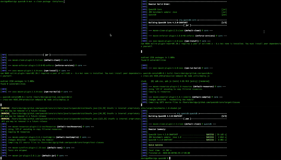
It builds really quickly due to the lack of external dependencies, so that is
great! Then all that's left to do is to start the server:
```shell
mkdir qdb
java -p core/target/questdb-5.0.5-SNAPSHOT.jar -m io.questdb/io.questdb.ServerMain -d qdb
```
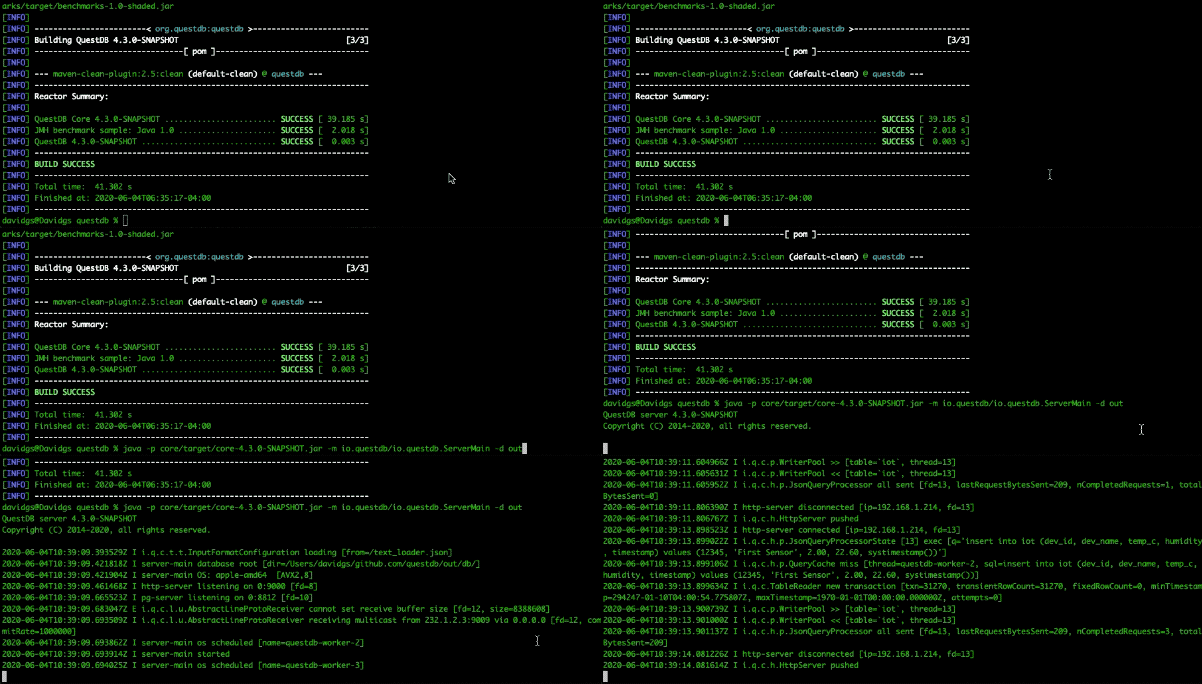
That is literally all there is to getting QuestDB built and running. But that's
just the first part. Now it's time to do something actually useful with it.
First, I'll need to create a table in QuestDB to store my IoT Data (A bit more
on this later, so store a pointer to this).
```
create table iot (
dev_id symbol index,
dev_name symbol index,
temperature double,
humidity double,
timestamp timestamp
) timestamp(timestamp) partition ...
### Things we learned about sums
**URL**: https://questdb.com/blog/2020/05/12/interesting-things-we-learned-about-sums/
**Description**: What we learned implementing Kahan and Neumaier compensated sum algorithms, benchmark and comparison with Clickhouse.
In the world of databases, benchmarking performance has always been the hottest
topic. Who is faster for data ingestion and queries? About a month ago we
announced a new release with SIMD aggregations on
[HackerNews](https://news.ycombinator.com/item?id=22803504) and
[Reddit](https://www.reddit.com/r/programming/comments/fwlk0k/questdb_using_simd_to_aggregate_billions_of/).
Fast. But were those results numerically accurate?
Speed is not everything. Some of the feedback we have received pointed us toward
the accuracy of our results. This is something typically overlooked in the
space, but our sums turned out to be "naive", with small errors for large
computations. By compounding a very small error over and over through a set of
operations, it can eventually become significant enough for people to start
worrying about it.
We then went on to include an accurate summation algorithm (such as "Kahan" and
"Neumaier" compensated sums). Now that we're doing the sums accurately, we
wanted to see how it affected performance. There is typically a trade-off
between speed and accuracy. However, by extracting even more performance out of
QuestDB (see below for how we did it), we managed to compute accurate sums as
fast as naive ones! Since comparisons to Clickhouse have been our most frequent
question, we have run the numbers and the result is:
[2x faster for summing 1bn doubles will nulls](#comparison-with-clickhouse).
All of this is included in our new
[release 4.2.1](https://github.com/questdb/questdb/releases/tag/4.2.1)
You can find our repository on [GitHub](https://github.com/questdb/questdb/).
All your
[issues](https://github.com/questdb/questdb/issues?q=is%3Aissue+is%3Aopen+sort%3Aupdated-desc),
[pull-requests](https://github.com/questdb/questdb/pulls?q=is%3Apr+is%3Aopen+sort%3Aupdated-desc)
and [stars](https://github.com/questdb/questdb/) are welcome 🙂.
How did we get there?
We used prefetch and co-routines techniques to pull data from RAM to cache in
paral...
### Aggregating billions of rows per second with SIMD
**URL**: https://questdb.com/blog/2020/04/02/using-simd-to-aggregate-billions-of-rows-per-second/
**Description**: How SIMD instructions make aggregations faster in QuestDB, including benchmark results and a comparison with Postgres.
[SIMD instructions](https://en.wikipedia.org/wiki/SIMD) are specific CPU
instruction sets for arithmetic calculations that use synthetic parallelization.
This approach allows us to perform the same calculations and operations on
numerous data points simultaneously. This post describes how SIMD works with
typical operation performance and describes additional optimizations we managed
to achieve.
What are SIMD operations?
Instead of spreading the work across CPU cores, SIMD performs vector operations
on multiple items using a **single** CPU instruction. In practice, if you were
to add 8 numbers together, SIMD does that in 1 operation instead of 8. We get
compounded performance improvements by combining SIMD with actual
parallelisation and spanning the work across CPUs.
QuestDB 4.2 introduces SIMD instructions, which made our aggregations faster by
100x! QuestDB is available open source (Apache 2.0) . If you like what we do,
please consider [starring our repo](https://github.com/questdb/questdb) and
following us on GitHub.
As of now, SIMD operations are available for non-keyed aggregation queries, such
as `select sum(value) from table`. In future releases, we will extend these to
keyed aggregations, for example `select key, sum(value) from table` (note the
intentional omission of `GROUP BY`). This will also result in ultrafast
aggregation for time bucketed queries using `SAMPLE BY`.
How much faster is SIMD?
We ran performance tests using 2 different CPUs: the
[Intel 8850H](https://ark.intel.com/content/www/us/en/ark/products/134899/intel-core-i7-8850h-processor-9m-cache-up-to-4-30-ghz.html)
and the AMD Ryzen 3900X. Both were running on 4 threads.
| Test | Query |
| --------------------------------- | ------------------------------------------------------------------------------------------------------- |
| sum of 1Bn doubles
QuestDB enables Energetech to process and aggregate financial market data
instantly. Learn more
}
/>
Cost-saving data architecture
Energetech's architecture efficiently ingests and processes vast amounts of
energy data from multiple providers. QuestDB plays a central role in storing and
querying time-series data with high performance and reliability.
The built-in [deduplication](/docs/concepts/deduplication/) and
[out-of-order](/blog/building-a-new-vector-based-storage-model/#the-problem-with-out-of-order-data)
handling capabilities of QuestDB simplify the data pipeline, enabling Energetech
to focus on delivering value to their clients. It also significantly limits
database growth, which results in both immediate and sustained cost savings.
```mermaid
flowchart TB
subgraph Providers
A[Market data]
end
subgraph Ingestion
B[Apache Kafka]
C[Price Index]
D[Forecasts]
end
subgraph Storage
E[QuestDB]
end
subgraph Processing
F[Prices API]
end
subgraph Serving
G[Grafana]
end
Providers --> Ingestion
Ingestion --> Storage
Storage --> Processing
Pr...
### HDFC Bank uses QuestDB for mule account detection across all major 25+ banking channels
**URL**: https://questdb.com/blog/hdfc-bank-uses-questdb-for-mule-account-detection/
**Description**: HDFC Bank, the largest private bank in India, uses QuestDB inside its in-house Real-Time Streaming Platform (RTSP) for real-time mule account detection, sustaining 5,000 to 7,000 transactions per second on a single instance with sub-second query latency.
[HDFC Bank](https://www.hdfcbank.com/) (HDFC Bank Limited) is one of India's
leading private sector banks, headquartered in Mumbai, Maharashtra. It is the
largest private bank in India by assets and market capitalization, and ranks
among the top global banks by market capitalization.
HDFC Bank mainly operates through three main segments: Retail Banking –
Individuals, small businesses; Wholesale Banking – Corporates, institutions; and
Treasury – Investments and financial markets.
Every transaction HDFC Bank processes goes through its transaction risk
monitoring system, and depending on the use case, suspicious patterns must be
identified within milliseconds. To support these real-time processing
requirements, HDFC Bank uses QuestDB as part of its in-house **Real-Time
Streaming Platform (RTSP)**, built to process high-volume streaming transaction
data with low latency. The current production implementation uses RTSP and
QuestDB for real-time **mule account detection**.
```info
A **money mule account** is a bank account used to receive and move funds
obtained through fraud or other crime, layering the money to disguise its
origin. The account holder may be a willing participant or an unwitting victim
recruited under false pretenses. Detecting mule accounts means spotting the
transaction patterns they leave behind, often spread across multiple channels.
```
The challenge: mule detection at national scale
Banks need to monitor every transaction in real time for patterns that indicate
fraudulent behaviour, or the suspicious account activity commonly associated
with mule accounts. For a bank the size of HDFC, that means evaluating thousands
of transactions per second, each one against multiple rule sets and models,
while meeting strict latency requirements.
Examples of the rules evaluated include:
- Is this merchant blacklisted?
- Has the account performed more than **X transactions exceeding ₹Y during the
last 15 minutes?**
- Have multiple transactions originated...
### OKX relies on QuestDB for exchange-wide analytics
**URL**: https://questdb.com/blog/okx-case-study/
**Description**: OKX is one of the world's largest cryptocurrency exchanges, handling billions of dollars in daily trading volume and serving millions of users worldwide.
OKX is one of the world's largest cryptocurrency exchanges, handling billions of
dollars in daily trading volume and serving millions of users worldwide. OKX's quantitative trading division requires real-time analytics, low-latency
ingestion, and continuous performance at scale.
To meet these requirements, OKX selected **QuestDB** as its core time series
database for market data analytics and trade execution analysis. They
replaced legacy systems that could no longer keep up with ingestion rates and
operational complexity, standardizing on QuestDB for its mix of high
performance, simplicity, and open architecture.
The Challenge
OKX handles streams of **high frequency market data**, capturing every quote,
order fill, and event happening on the exchange. Each system must process large
volumes of messages per second while ensuring data integrity and enabling fast
query access for analytics.
Before adopting QuestDB, OKX used **InfluxDB** to store internal market data.
Over time, ingestion performance degraded as data volumes increased, which led
to operational friction and frequent re-tuning of clusters. Data retention had
to be limited, query latency grew, and debugging slowdowns became costly.
OKX needed a system that could:
- Ingest high-frequency market events without bottlenecks
- Offer SQL capabilities for rapid analytics and monitoring
- Integrate easily with Apache Kafka and Grafana
- Deploy in their own cloud environments for data locality
- Support ~1 week hot retention while archiving raw data to object storage
Key Components
**Apache Kafka integration:** OKX publishes internal market data and order fill
streams to Kafka. QuestDB ingests those streams and runs behind a load balancer,
allowing multiple instances to process data in parallel for scalability and
resilience.
**Fast market data ingestion:** QuestDB's high-throughput endpoint provides ultra-fast ingestion from
internal services while keeping writes schema-aware and simple to operate.
**Gra...
### One Trading runs a regulated 24/7 futures exchange on QuestDB
**URL**: https://questdb.com/blog/one-trading-runs-a-regulated-24-7-futures-exchange-on-questdb/
**Description**: One Trading runs a regulated 24/7 futures exchange on QuestDB: 1.8M orders/sec, 5M+ rows/sec ingestion, real-time surveillance, room to scale.
[One Trading](https://onetrading.com/) is a regulated European derivatives
exchange operating under MiFID II and MiCAR. They offer derivatives
including dated futures across crypto and equity markets, serving retail,
professional, and institutional clients across the EEA with full cross
margining and portfolio margining.
One Trading is also the first venue to bring 24/7 central limit order book
(CLOB) trading to equity futures, a round-the-clock product that
only works if the data platform behind it can keep pace without interruption.
Their matching engine sustains 1.8 million orders per second, with round-trip
latency held under 200 microseconds through close work with AWS on [cloud-native
colocation](https://aws.amazon.com/blogs/industries/one-trading-exchange-and-aws-cloud-native-colocation-for-crypto-trading/).
Everything downstream depends on the data platform keeping up.
The journey to QuestDB
One Trading's initial stack used Amazon DynamoDB and RDS, and later raw NDJSON
files on S3 to keep up with write volume. These worked early on, but as trading
activity grew the exchange quickly needed a purpose-built, high-performance
database: one that could ingest streaming market data at full speed, serve
queries in real time, and scale under ever-growing volumes.
Evaluating alternatives
One Trading evaluated several databases before choosing QuestDB:
| System | Issue | Limitation |
|--------|-------|------------|
| TimescaleDB | Performance | Could not sustain high-volume ingestion.
Lacks capital-markets SQL primitives |
| Amazon Timestream
for LiveAnalytics | Cost and performance | Now deprecated by AWS. Cost model
unsuitable, performance a concern |
| InfluxDB | Performance | Could not sustain high-volume ingestion.
Slow on high-cardinality data |
What worked: QuestDB
QuestDB met the requirements the previous architectures could not satisfy
simultaneously:
Results
All from a single data platform. The use cases running against this
deploym...
### Reflexivity switched from InfluxDB to QuestDB
**URL**: https://questdb.com/blog/reflexivity-case-study/
**Description**: Reflexivity is a SaaS company that uses QuestDB to provide state-of-the-art AI technology to help investors turn Big Data into investment insights.
[Reflexivity](https://www.reflexivity.com/) is a SaaS company that uses QuestDB
to provide AI-powered investment insights from all data that moves markets.
Reflexivity uses AI and machine learning to help investors extract signals from
vast amounts of market data. The platform ingests and processes billions of data
points, including prices, fundamentals and sentiment, then distills them into
actionable alerts such as "Analyst expectations are turning negative for AAPL;
historically this pattern precedes outperformance of the stock."
This workload relies on a continuous stream of time series data that must be
stored efficiently and queried quickly by downstream models. Every step of the
pipeline needs to be optimised, from ingestion to historical analysis, in order
to keep query latency low while controlling infrastructure cost.
Scaling challenges with InfluxDB
Before adopting QuestDB, Reflexivity experimented with several databases,
including MongoDB, Cassandra and TimescaleDB. After extensive testing they
initially standardised on InfluxDB, which provided the best performance at the
time. As the company and data volumes grew, however, the InfluxDB deployment
became increasingly expensive and difficult to operate.
The production cluster ran on four m4.2xlarge instances with 128 GiB of RAM.
Memory usage across the cluster frequently sat above 80 percent and regularly
spiked to 100 percent several times per week. When the team projected
infrastructure requirements for future growth, it became clear that InfluxDB
would not be a viable option at scale.
Selecting a new time series database
When evaluating alternatives, Reflexivity defined a set of practical questions
that any replacement needed to answer positively:
- Can existing data be moved seamlessly and quickly?
- Can the team query a representative sample of data with response times at
least as good as InfluxDB?
- Can new data be ingested without disruption?
- Can new time series be created on the fly as...
### Virtual Global Trading leverages QuestDB for efficient energy data management
**URL**: https://questdb.com/blog/virtual-global-trading-case-study/
**Description**: Virtual Global Trading uses QuestDB to manage time-series data for energy production and consumption, enabling dynamic pricing and efficient energy distribution across smart meters, power plants, and grid infrastructure.
[Virtual Global Trading](https://www.vgt.energy/) uses QuestDB to manage
time-series data for energy production and consumption, enabling dynamic pricing
and efficient energy distribution across smart meters, power plants, and grid
infrastructure.
Efficient energy data management
Virtual Global Trading leverages QuestDB to receive data from a broad array of
smart meters, power plants, sensors, and other devices that monitor energy grid
usage. Data is time-bound for billing and tracking purposes, and a dedicated
time-series database ensures clean, timely arrival of the information required
for downstream analytics.
SQL, clean and simple
Virtual Global Trading uses powerful SQL queries to manage and aggregate
time-series data efficiently. Time-series extensions such as `SAMPLE BY` enhance
the precision of these queries, enabling better data handling and visualization.
Data from various sensors arrives in real time, then is processed and aggregated
by time. This supports dynamic pricing calculations and real-time information
for both customers and internal applications.
The following query illustrates how deduplication, aggregation, and
calendar-aligned sampling work together:
- A subquery filters and deduplicates data by `measuredUTC` and `importedUTC`
using `LATEST ON`.
- The outer query aggregates the filtered data, sums `value`, and computes the
minimum of `measuredUTC` and `importedUTC`.
- `SAMPLE BY` groups the data into yearly intervals and aligns it to the
calendar in the `'Europe/Zurich'` time zone.
```questdb-sql
SELECT
datapointName,
meteringPointID,
source,
sourceID,
interval,
status,
MIN(measuredUTC) AS measuredUTC,
MIN(importedUTC) AS importedUTC,
SUM(value) AS value
FROM
(
SELECT
datapointName,
meteringPointID,
value,
source,
sourceID,
interval,
status,
measuredUTC,
importedUTC
FROM
WHERE
measuredUTC >= '2015-10-31T00:00:00.000000Z'
AND measuredUTC < '2025-1...
### XRP Ledger uses QuestDB for real-time blockchain analytics
**URL**: https://questdb.com/blog/xrp-ledger-case-study/
**Description**: The Inclusive Financial Technology Foundation needs fast, modern tooling to keep up with XRP Ledger and the Xahau network as a rapidly evolving L1 blockchain with over 1500 applications.
The
[Inclusive Financial Technology Foundation (previously XRP Ledger Foundation)](https://inftf.org/)
needs fast, modern tooling for the [XRP Ledger](https://xrpl.org/), a rapidly
evolving L1 blockchain with over 1500 applications. The ecosystem, including the
[Xahau](https://xahau.network/) smart contract sidechain, continues to grow.
Handling vast transaction data
A large amount of transaction data is being processed on the XRP Ledger and the
Xahau Network.
They use QuestDB to provide an API that formats transaction data based on
transaction time, enabling user-facing applications to retrieve data in an
organized, human-friendly format.
QuestDB enables the XRP Ledger to process vast amounts of transaction data
instantly.{" "}
Learn more
}
/>
Why XRP Ledger chose QuestDB
Daniel Siedentopf, Technical Team Lead, explains that the XRP Ledger Foundation
needed a robust database to take over the role previously filled by their former
engine, which had been discontinued because of its high operational cost. The
replacement had to handle large volumes of time series data generated by
blockchain transactions, support complex queries, and deliver high reliability
and performance.
The team evaluated several time series databases, including InfluxDB and
TimescaleDB, using performance benchmarks as the main decision factor. QuestDB
was selected because it delivered better query speed and data throughput than
the alternatives, which is critical for XRPL workloads where real-time
processing and fast access to historical data are essential.
Open source was another important requirement. QuestDB's open source model
aligned with the foundation's operational philosophy and gave the team
flexibility as their architecture evolves.
In production, QuestDB now powers complex qu...
## Glossary
### ACID Table
**Description**: Comprehensive overview of ACID tables in data systems. Learn how these database tables guarantee data consistency and reliability through Atomicity, Consistency, Isolation, and Durability properties.
An ACID table is a database table that guarantees the four fundamental properties of transaction processing: Atomicity, Consistency, Isolation, and Durability. In modern data architectures, ACID tables are crucial for maintaining data integrity, especially in data lake and [lakehouse architecture](/glossary/lakehouse-architecture/) implementations.
Understanding ACID properties in tables
ACID tables implement four key guarantees:
1. **Atomicity**: All operations within a transaction either complete fully or not at all
2. **Consistency**: Data remains valid according to defined rules
3. **Isolation**: Concurrent transactions don't interfere with each other
4. **Durability**: Committed changes persist even during system failures
```mermaid
graph TD
A[Transaction Start] --> B{Atomic Operation}
B -->|Success| C[Commit]
B -->|Failure| D[Rollback]
C --> E[Durable State]
D --> F[Previous State]
```
Implementation in modern data systems
ACID table...
### Adaptive Trading Algorithms
**Description**: Comprehensive overview of adaptive trading algorithms in financial markets. Learn how these sophisticated systems dynamically adjust their strategies based on changing market conditions.
Adaptive trading algorithms are automated trading systems that dynamically modify their behavior and parameters in response to changing market conditions. These algorithms use real-time feedback loops to optimize their trading strategies, adjusting factors such as order timing, size, and placement based on observed market dynamics and execution performance.
Core principles of adaptive trading algorithms
Adaptive trading algorithms operate on the principle of continuous learning and adjustment. Unlike static algorithms that follow fixed rules, adaptive systems incorporate feedback mechanisms to evolve their strategies based on:
- Market microstructure changes
- Execution performance metrics
- Liquidity dynamics
- Price volatility patterns
- Trading volume profiles
These algorithms align closely with the Adaptive Market Hypothesis, which suggests that market efficiency and trading opportunities evolve over time.
Adaptation mechanisms
Real-time parameter adjustm...
### AI-Augmented Portfolio Optimization
**Description**: Comprehensive overview of AI-augmented portfolio optimization in financial markets. Learn how artificial intelligence enhances modern portfolio theory and improves investment outcomes through advanced data analysis and adaptive strategies.
AI-augmented portfolio optimization combines traditional portfolio management techniques with artificial intelligence to enhance investment decision-making. This approach leverages machine learning algorithms and advanced data analytics to improve asset allocation, risk management, and return optimization beyond conventional mean-variance optimization methods.
How AI enhances portfolio optimization
AI-augmented portfolio optimization extends traditional portfolio theory by incorporating:
1. Dynamic asset allocation that adapts to changing market conditions
2. Complex pattern recognition in market behavior
3. Multi-factor optimization across numerous constraints
4. Real-time portfolio rebalancing signals
5. Alternative data integration for enhanced market insights
The integration of AI enables portfolio managers to process vast amounts of structured and unstructured data, identifying subtle relationships that traditional statistical methods might miss.
Key comp...
### Alert Thresholding
**Description**: Comprehensive overview of alert thresholding in time-series monitoring. Learn how this critical technique helps detect anomalies and trigger notifications based on predefined conditions in time-series data.
Alert thresholding is a monitoring technique that triggers notifications when time-series metrics cross predefined boundary values. It enables automated detection of anomalies, performance issues, or business-critical conditions by comparing real-time data against established thresholds.
Understanding alert thresholding fundamentals
Alert thresholding establishes boundaries for acceptable behavior in time-series data. When values exceed these boundaries, the system generates alerts to notify stakeholders. This process involves several key components:
1. Threshold definition - Static or dynamic values that represent boundaries
2. Comparison logic - Rules for evaluating metrics against thresholds
3. Alert generation - Creation and delivery of notifications
4. Alert state management - Tracking of active and resolved alerts
```mermaid
flowchart LR
A[Time-series Data] --> B[Threshold Check]
B --> C{Condition Met?}
C -->|Yes| D[Generate Alert]
C -->|N...
### Algorithmic Execution Strategies
**Description**: Algorithmic execution strategies split large orders into smaller pieces executed by rules over time, cutting market impact and transaction costs across venues.
Algorithmic execution strategies are automated trading approaches that break large orders into smaller pieces and execute them over time according to predefined rules and market conditions. These strategies aim to minimize market impact, reduce transaction costs, and achieve optimal execution prices while managing various risks.
Core components of execution algorithms
Execution algorithms incorporate several key elements to achieve their objectives:
- Order scheduling: Determining the optimal timing and size of child orders
- Venue selection: Choosing where to route orders based on liquidity and costs
- Price limits: Setting boundaries to control execution prices
- Market impact estimation: Modeling how trades affect market prices
- Risk controls: Monitoring and managing execution risks
Common execution strategy types
Time-Weighted Average Price (TWAP)
[TWAP](/glossary/time-weighted-average-price-twap/) strategies divide orders into equal-sized pieces and exe...
### Algorithmic Portfolio Rebalancing
**Description**: Comprehensive overview of algorithmic portfolio rebalancing in financial markets. Learn how automated systems maintain target allocations, manage risk, and optimize trading costs across multiple asset classes.
Algorithmic portfolio rebalancing refers to the automated process of adjusting portfolio holdings to maintain desired asset allocations and risk targets. These systems use quantitative methods to optimize trade execution while minimizing market impact and transaction costs.
Understanding algorithmic portfolio rebalancing
Algorithmic portfolio rebalancing combines [execution algorithms](/glossary/execution-algorithms/) with portfolio optimization techniques to systematically maintain target asset allocations. As market movements cause portfolio weights to drift from their targets, rebalancing algorithms calculate required trades and execute them efficiently.
The process typically involves:
1. Monitoring portfolio drift from targets
2. Calculating optimal rebalancing trades
3. Executing trades while managing costs
4. Verifying post-trade allocations
```mermaid
graph TD
A[Monitor Portfolio Drift] --> B[Calculate Target Trades]
B --> C[Cost Analysis]
C...
### Algorithmic Risk Controls
**Description**: Algorithmic risk controls are automated guardrails that monitor trading, block erroneous orders, enforce position limits, and keep automated systems compliant.
Algorithmic risk controls are automated systems and procedures designed to monitor, detect, and prevent potentially dangerous trading behavior in electronic trading environments. These controls act as guardrails for [algorithmic trading](/glossary/algorithmic-trading/) systems, helping to prevent erroneous trades, maintain position limits, and ensure compliance with regulatory requirements.
Core components of algorithmic risk controls
Pre-trade risk checks
Pre-trade risk controls validate orders before they enter the market, examining factors such as:
- Position limits and exposure thresholds
- Order size and price boundaries
- Trading frequency and order flow rates
- Available capital and margin requirements
```mermaid
flowchart TD
A[Incoming Order] --> B{Pre-trade Check}
B -->|Pass| C[Submit to Market]
B -->|Fail| D[Reject Order]
C --> E[Post-trade Monitoring]
E -->|Risk Threshold Breach| F[Emergency Actions]
```
Real-time monitoring and ...
### Algorithmic Trading
**Description**: Comprehensive overview of algorithmic trading in financial markets. Learn how automated trading strategies execute orders using predefined rules, mathematical models, and real-time market data analysis.
Algorithmic trading is the automated execution of trading decisions using computer programs that follow predefined rules and mathematical models. These systems analyze market data in real-time, make trading decisions, and automatically execute orders without direct human intervention. Algorithmic trading accounts for a significant portion of trading volume in modern financial markets.
Core components of algorithmic trading
Algorithmic trading systems consist of several interconnected components that work together to implement trading strategies:
1. Data processing engine - Ingests and normalizes real-time [market data](/capital-markets/) from multiple sources
2. Strategy engine - Analyzes data and generates trading signals based on predefined rules
3. Risk management module - Enforces position limits and [pre-trade risk checks](/glossary/pre-trade-risk-checks/)
4. Order execution engine - Implements [order execution algorithms](/glossary/order-execution-algorith...
### Anomaly Detection in Industrial Systems
**Description**: Comprehensive overview of anomaly detection in industrial systems. Learn how organizations leverage time-series data analysis to identify equipment failures, process deviations, and operational irregularities.
Anomaly detection in industrial systems refers to the automated identification of unusual patterns, unexpected behavior, or deviations from normal operating conditions in manufacturing and process control environments. This critical capability helps organizations prevent equipment failures, maintain product quality, and optimize operational efficiency through real-time monitoring and analysis of time-series data from sensors and control systems.
Understanding industrial anomaly detection
Industrial anomaly detection systems analyze continuous streams of sensor data to identify patterns that deviate from expected behavior. These systems typically monitor multiple parameters simultaneously, including:
- Temperature and pressure readings
- Vibration patterns
- Power consumption
- Flow rates
- Chemical composition measurements
- Production line speeds
```mermaid
graph TD
A[Sensor Data Collection] --> B[Data Preprocessing]
B --> C[Normal Pattern Learning]
...
### Anomaly Detection in Time Series Data
**Description**: Comprehensive overview of anomaly detection in time series data. Learn how organizations identify unusual patterns and outliers in sequential data to detect anomalies, prevent system failures, and maintain market integrity.
Anomaly detection in time series data is the process of identifying unusual patterns, outliers, or unexpected behavior in sequential data points ordered by time. In financial markets and industrial systems, this capability is crucial for detecting market manipulation, system failures, and trading anomalies that could indicate risks or opportunities.
Understanding time series anomalies
Time series anomalies typically fall into three main categories:
1. Point anomalies: Single data points that deviate significantly from the expected range
2. Contextual anomalies: Data points that are unusual in a specific context or time window
3. Pattern anomalies: Sequences of points that form unusual patterns
For example, in financial markets, a sudden price spike might be a point anomaly, while unusual trading volumes during typically quiet periods represent contextual anomalies. Pattern anomalies could include irregular order book patterns that might indicate market manipula...
### Anomaly Score
**Description**: Comprehensive overview of anomaly scores in time-series analysis. Learn how these numerical metrics quantify the degree of abnormality in data points and their crucial role in anomaly detection systems.
An anomaly score is a numerical value that quantifies how much a data point or pattern deviates from expected normal behavior. In time-series analysis, these scores help identify and rank potential anomalies, enabling automated detection systems to prioritize and classify unusual events.
How anomaly scores work
Anomaly scores measure the degree of deviation from normal patterns using statistical or machine learning methods. The higher the score, the more likely a data point represents an anomaly. These scores typically account for multiple factors:
- Historical patterns and seasonality
- Statistical distributions
- Multiple dimensions or metrics
- Context-specific thresholds
```python
Simplified example of Z-score based anomaly scoring
def calculate_anomaly_score(value, mean, std_dev):
return abs((value - mean) / std_dev)
```
Common scoring methods
Statistical approaches
Statistical methods calculate anomaly scores based on probability distributions and ...
### Apache Iceberg
**Description**: Comprehensive overview of Apache Iceberg, an open table format for huge analytic datasets. Learn how Iceberg manages large-scale data lake tables with atomic transactions, schema evolution, and time travel capabilities.
Apache Iceberg is an open table format designed for massive analytic datasets. It provides transactional guarantees, schema evolution, and time travel capabilities while managing large-scale data lake tables. Iceberg enables reliable, high-performance access to data lake storage through its table format specification.
How Apache Iceberg works
Iceberg manages tables through a series of immutable snapshots, each representing a complete version of the table. This approach enables atomic transactions and time travel queries while maintaining performance at scale.
```mermaid
graph TD
A[Table Metadata] --> B[Current Snapshot]
A --> C[Previous Snapshots]
B --> D[Manifest Lists]
D --> E[Manifests]
E --> F[Data Files]
```
Key features and capabilities
Schema evolution
Iceberg supports in-place schema evolution, allowing columns to be added, removed, or reordered without copying data. This flexibility is crucial for time-series data management where ...
### Apache Parquet, What It Is and Why to Use It
**Description**: Apache Parquet is a columnar storage format. See how it works, its compression and query benefits, and who gains most, with clear examples.
Apache Parquet is a columnar storage file format designed for efficient data
processing and storage. It was developed to handle large-scale data processing
and analytics through better performance and more efficient data compression. It
was initially created by engineers at Twitter and Cloudera, and was released in
March 2013 as an [open-source project](https://github.com/apache/parquet-format)
under the Apache Software Foundation.
We'll unpack what it is and compare its features to other storage formats.
Why Parquet?
The motivation behind Parquet was to address the limitations of existing storage
formats, particularly for "big data" processing. Twitter needed a more efficient
and performant way to store and process large-scale datasets, especially for
analytic queries.
According to the excellent article
"[The birth of Parquet](https://sympathetic.ink/2024/01/24/Chapter-1-The-birth-of-Parquet.html)"
by Julien Le Dem, Parquet was born out of the "Red Elm" system. The goal wa...
### Append-only Log
**Description**: Append-only logs add records only at the end, never editing or deleting them, giving time-series databases and event streams durable, ordered data.
An append-only log is a data structure that only allows new records to be added to the end of the sequence, never modified or deleted. This immutable design pattern is fundamental to time-series databases, event sourcing systems, and distributed data platforms, providing a reliable foundation for data consistency and real-time streaming.
How append-only logs work
Append-only logs store data sequentially, with each new record receiving a unique, monotonically increasing identifier. This sequential nature creates a natural timeline of events, making them ideal for:
- Time-series data storage
- Event sourcing
- Transaction logging
- Change data capture (CDC)
```mermaid
graph LR
A[New Event] --> B[Log Head]
B --> C[Recent Events]
C --> D[Historical Events]
D --> E[Log Tail]
```
Benefits of append-only design
Data integrity
Since existing records cannot be modified, append-only logs provide natural audit trails and make it easier to maintain data c...
### Append-only Storage
**Description**: Append-only storage writes new records sequentially without modifying old ones, giving time-series databases fast ingestion, immutability, and simple recovery.
Append-only storage is a database design pattern where new data is exclusively added to the end of existing data structures, without modifying or deleting existing records. This approach is particularly well-suited for time-series databases, offering superior write performance, data integrity, and simplified recovery mechanisms.
How append-only storage works
Append-only storage treats data as an immutable log of events, where each new record is written sequentially after the previous one. This pattern aligns naturally with time-series data, where newer events occur later in time and are written in chronological order.
```mermaid
graph LR
A[New Data] --> B[Write Buffer]
B --> C[Append to Storage]
C --> D[Commit]
```
The sequential nature of writes eliminates the need for random disk access during ingestion, leading to significantly improved write performance.
Benefits for time-series workloads
Optimized write performance
Since data is only written ...
### Atomic Transactions in Financial Systems
**Description**: Comprehensive overview of atomic transactions in financial markets and trading systems. Learn how atomic operations ensure data consistency and reliability in critical financial operations.
Atomic transactions are operations that must be executed as a single, indivisible unit where either all steps complete successfully or none of them do. In financial systems, atomic transactions are crucial for maintaining data consistency and preventing partial updates that could lead to incorrect balances, failed trades, or mismatched positions.
Understanding atomic transactions in finance
In financial markets, atomic transactions are essential for maintaining the integrity of trading operations. For example, when executing a trade, multiple steps must occur atomically:
1. Verify available funds/positions
2. Place the order
3. Update account balances
4. Record the transaction
If any step fails, the entire transaction must be rolled back to prevent inconsistencies. This "all-or-nothing" property is fundamental to financial system reliability.
Applications in market operations
Order execution
In [algorithmic trading](/glossary/algorithmic-trading/), atomic tr...
### Autocorrelation Function
**Description**: Comprehensive overview of autocorrelation function (ACF) in time-series analysis. Learn how this statistical tool measures serial correlation and helps identify patterns in sequential data.
The autocorrelation function (ACF) measures the correlation between observations at different time lags in a time series. It reveals patterns, seasonality, and dependencies in sequential data by quantifying how similar the series is to itself when shifted by various time intervals.
Understanding autocorrelation function
The autocorrelation function is a fundamental tool in [time-series analysis](/glossary/time-series-analysis/) that measures the linear correlation between observations separated by specific time lags. For a time series $Y_t$, the ACF at lag $k$ is defined as:
$$ \rho(k) = \frac{\mathbb{E}[(Y_t - \mu)(Y_{t+k} - \mu)]}{\sigma^2} $$
Where:
- $\mu$ is the mean of the series
- $\sigma^2$ is the variance
- $k$ is the lag value
- $\mathbb{E}$ denotes expected value
Properties and interpretation
Key characteristics
1. **Range**: ACF values fall between -1 and 1
- +1 indicates perfect positive correlation
- -1 indicates perfect negative correlat...
### Avro
**Description**: Comprehensive overview of Apache Avro data serialization. Learn how this compact binary format enables efficient data exchange and schema evolution in time-series systems.
Apache Avro is a data serialization system that provides a compact, fast binary format with integrated schema support. Designed for efficient data exchange in big data systems, Avro combines schema evolution capabilities with type safety while maintaining high performance.
How Avro works
Avro serializes data using a schema-based approach. Each Avro record contains both the data and its schema definition, enabling self-describing data streams. The schema is defined using JSON, while the data itself is stored in a compact binary format.
```mermaid
graph LR
A[JSON Schema] --> B[Avro Serializer]
C[Application Data] --> B
B --> D[Binary Avro Data]
D --> E[Avro Deserializer]
E --> F[Reconstructed Data]
```
Schema evolution capabilities
One of Avro's key strengths is its support for schema evolution, allowing data producers and consumers to work with different schema versions. This is particularly valuable in time-series systems where data structu...
### Backfill
**Description**: Comprehensive overview of backfill in time-series databases. Learn how backfilling enables historical data loading, supports data corrections, and maintains data completeness in time-series systems.
Backfill refers to the process of loading or updating historical data in a time-series database. This operation is essential for filling gaps in data history, correcting errors, or initializing systems with historical records. Backfilling must handle out-of-order data ingestion while maintaining data consistency and system performance.
Understanding backfill operations
Backfill operations are crucial for maintaining complete and accurate time-series data. Unlike real-time data ingestion, backfilling involves processing historical data that may arrive out of chronological order or need to be updated retroactively.
```mermaid
flowchart LR
A[Historical Data Source] --> B[Backfill Process]
B --> C[Data Validation]
C --> D[Time-series DB]
D --> E[Updated History]
```
Common backfill scenarios
Data recovery and correction
When systems experience downtime or data errors, backfilling helps restore data integrity by:
- Filling gaps from service interrup...
### Backpressure Handling
**Description**: Comprehensive overview of backpressure handling in data systems. Learn how this flow control mechanism prevents system overload and ensures reliable data processing in high-volume time-series applications.
Backpressure handling refers to mechanisms that manage and control data flow when a system's consumption rate cannot match its input rate. It's a critical flow control pattern that prevents system overload by regulating data transmission between components, ensuring system stability and reliable data processing.
Understanding backpressure in data systems
Backpressure occurs when a system component receives data faster than it can process it. Like water pressure in a pipe, data "pressure" builds up when there's a mismatch between input and processing rates. Effective backpressure handling implements strategies to manage this pressure and maintain system stability.
```mermaid
graph LR
A[Fast Producer] -->|High Volume Data| B[Buffer]
B -->|Controlled Flow| C[Slower Consumer]
C -->|Feedback Signal| A
```
Common backpressure handling strategies
Buffer-based approaches
Systems can implement buffers to temporarily store incoming data when processing canno...
### Backtesting
**Description**: Backtesting evaluates trading strategies by simulating their performance on historical market data, gauging viability before risking real capital live.
Backtesting is a critical methodology in quantitative finance that evaluates trading strategies by simulating their performance using historical market data. This process helps traders and analysts assess the viability of trading strategies before risking real capital in live markets.
Core concepts of backtesting
Backtesting simulates trading decisions using historical price data and market conditions to evaluate how a strategy would have performed in the past. The process involves reconstructing market conditions and applying trading rules systematically to generate performance metrics.
Key components include:
- Historical market data and pricing
- Trading strategy rules and parameters
- Transaction cost modeling
- Position sizing and risk management rules
- Performance measurement metrics
Types of backtesting approaches
Point-in-time backtesting
This method uses only data that would have been available at each historical moment, preventing look-ahead bias. I...
### BASE Model
**Description**: Comprehensive overview of the BASE model in distributed databases. Learn how this consistency model prioritizes availability and scalability over strict consistency, making it particularly relevant for time-series systems.
The BASE model (Basically Available, Soft state, Eventually consistent) is a database design philosophy that favors availability and performance over immediate consistency. Unlike the ACID model's strict guarantees, BASE accepts that database state may be in flux, making it particularly suitable for distributed time-series systems where high-speed ingestion and scalability are critical.
Understanding the BASE principles
The BASE model consists of three core principles:
1. **Basically Available**: The system guarantees availability of data, even in the presence of failures, though responses may be incomplete or in flux.
2. **Soft state**: The system's state may change over time, even without input, due to eventual consistency requirements.
3. **Eventually consistent**: The system will become consistent over time, given that the system processes all updates.
```mermaid
flowchart LR
A[Write Request] --> B[Node 1]
A --> C[Node 2]
A --> D[Node 3]
B...
### Batch Ingestion
**Description**: Comprehensive overview of batch ingestion in time-series databases. Learn how batch processing enables efficient loading of historical data, the tradeoffs between batch and streaming ingestion, and best practices for optimizing batch operations.
Batch ingestion is a data loading pattern where records are collected into
groups and processed together in discrete intervals, rather than handled
individually in real-time. This approach is particularly important for
time-series databases, offering efficient ways to load historical data,
perform bulk updates, and optimize resource usage.
How batch ingestion works
Batch ingestion aggregates data into chunks before processing, following a
collect-then-process pattern. This differs from
[real-time ingestion](/glossary/real-time-data-ingestion/) where records are
processed immediately as they arrive. The batch process typically involves:
1. Data collection and staging
2. Validation and transformation
3. Bulk loading into the target database
4. Post-load verification and cleanup
```mermaid
flowchart LR
A[Data Sources] --> B[Collection Buffer]
B --> C[Batch Processing]
C --> D[Validation]
D --> E[Bulk Load]
E --> F[Database]
```
Advan...
### Batch vs. Stream Processing
**Description**: Comprehensive overview of batch and stream processing in time-series data systems. Learn how these fundamental data processing paradigms differ and their implications for financial markets and real-time analytics.
Batch and stream processing represent two distinct approaches to data processing. Batch processing handles data in large, fixed chunks at scheduled intervals, while stream processing deals with data continuously in real-time as it arrives. The choice between these methods significantly impacts system architecture, latency, and resource utilization.
Understanding batch processing
Batch processing involves collecting data over a period and processing it as a group or "batch." This approach is analogous to processing trades at the end of a trading day or calculating [portfolio rebalancing](/glossary/portfolio-rebalancing-algorithms/) adjustments overnight.
Key characteristics of batch processing:
- Fixed processing windows
- High throughput for large datasets
- Predictable resource allocation
- Lower operational complexity
- Built-in error recovery mechanisms
```mermaid
graph TD
A[Data Collection] --> B[Data Storage]
B --> C[Batch Window]
C --> D[Proce...
### Bayesian Inference in Quant Trading
**Description**: Bayesian inference in quant trading updates market beliefs as new data arrives, combining prior knowledge with live data for more robust trading decisions.
Bayesian inference in quantitative trading is a probabilistic framework that enables systematic updating of market beliefs and trading strategies as new information becomes available. It provides a rigorous mathematical foundation for combining prior knowledge with real-time market data to generate more robust trading decisions.
Understanding Bayesian inference in trading
Bayesian inference provides a mathematical framework for updating probabilistic beliefs about market conditions as new data arrives. Unlike traditional [statistical risk models](/glossary/statistical-risk-models/), Bayesian approaches explicitly model uncertainty and allow traders to incorporate prior knowledge into their analysis.
The core components include:
1. Prior distributions - Initial beliefs about market parameters
2. Likelihood functions - Models of how market data is generated
3. Posterior distributions - Updated beliefs after observing new data
Applications in quantitative trading...
### Benchmark Index
**Description**: Comprehensive overview of benchmark indices in financial markets. Learn how these standardized market measures serve as performance yardsticks and underlie countless financial products.
A benchmark index is a standardized measure that tracks the performance of a specific market segment or investment strategy. It serves as a reference point for evaluating investment performance, constructing financial products, and making asset allocation decisions. Common examples include the S&P 500 for U.S. large-cap stocks and the Bloomberg Global Aggregate for fixed income markets.
Core functions of benchmark indices
Benchmark indices serve multiple critical functions in financial markets. They provide a standardized way to measure market performance, enable performance attribution analysis, and form the basis for index-linked investment products like ETFs. The construction and maintenance of these indices follow strict methodologies to ensure representativeness and reliability.
```mermaid
graph TD
A[Benchmark Index] --> B[Performance Measurement]
A --> C[Product Creation]
A --> D[Risk Analysis]
B --> E[Portfolio Tracking]
B --> F[Attrib...
### Binomial Option Pricing Model
**Description**: The Binomial Option Pricing Model values options using a discrete-time tree of up and down price moves, discounting payoffs under risk-neutral probabilities.
The Binomial Option Pricing Model is a discrete-time framework for valuing options by modeling multiple possible price paths through a binary tree structure. Each node represents a possible asset price, with branches representing up or down movements, ultimately leading to a distribution of potential option payoffs that can be discounted to determine present value.
Core concepts of the binomial model
The binomial model assumes that an asset price can only move up or down by specific factors during each time step. This simplified approach creates a powerful framework for understanding option pricing and replication through dynamic hedging.
Key parameters include:
- Up factor (u): The multiplicative factor for upward price movements
- Down factor (d): The multiplicative factor for downward price movements
- Risk-free rate (r): The interest rate used for discounting
- Probability (p): Risk-neutral probability of an upward movement
The model's mathematical foundati...
### Black-Scholes Model for Option Pricing
**Description**: The Black-Scholes Model prices European options with a closed-form formula using underlying price, strike, time, risk-free rate, and volatility.
The Black-Scholes Model is a mathematical framework for pricing European-style options. Published in 1973 by Fischer Black, Myron Scholes, and Robert Merton, it provides a closed-form solution for determining theoretical option prices based on variables including the underlying price, strike price, time to expiration, risk-free rate, and volatility.
Core equation and assumptions
The Black-Scholes partial differential equation (PDE) for option pricing is:
$\frac{\partial V}{\partial t} + \frac{1}{2}\sigma^2S^2\frac{\partial^2 V}{\partial S^2} + rS\frac{\partial V}{\partial S} - rV = 0$
Where:
- $V$ is the option value
- $S$ is the underlying asset price
- $t$ is time
- $r$ is the risk-free rate
- $\sigma$ is volatility
The model makes several key assumptions:
- European-style options (no early exercise)
- Log-normal distribution of underlying returns
- Constant volatility and risk-free rate
- No dividends
- No transaction costs or taxes
- Continuous trading
Cl...
### Black-Scholes Model Limitations
**Description**: Black-Scholes model limitations expose gaps between its assumptions and real markets, from constant volatility to frictionless trading, skewing option prices.
The Black-Scholes model's limitations highlight critical gaps between theoretical assumptions and real market behavior. While revolutionary for options pricing, the model's simplifying assumptions about market conditions, volatility behavior, and trading mechanics can lead to significant pricing discrepancies in practice.
Understanding the model's core constraints
The Black-Scholes model, while foundational to modern options pricing, operates under several idealized assumptions that diverge from real market conditions. These limitations become particularly important for trading systems and risk management frameworks that rely on the model's outputs.
```mermaid
graph TD
A[Black-Scholes Assumptions] --> B[Constant Volatility]
A --> C[Log-Normal Distribution]
A --> D[Continuous Trading]
A --> E[No Transaction Costs]
B --> F[Volatility Smile]
C --> G[Fat Tails]
D --> H[Market Gaps]
E --> I[Real Costs]
```
Impact on volatility modelin...
### Block Trade Reporting
**Description**: Comprehensive overview of block trade reporting in financial markets. Learn how large trades are reported to market participants while managing information leakage and market impact.
Block trade reporting refers to the regulatory requirements and market practices for disclosing large-scale securities transactions. These specialized reporting mechanisms balance market transparency with the need to minimize market impact for institutional-sized trades.
Understanding block trade reporting
Block trade reporting encompasses the rules, systems, and practices for disclosing large securities transactions to the market. Block trades are substantial orders that exceed normal market size and require special handling to avoid significant market impact. The reporting framework must balance two competing interests: market transparency and the legitimate need to protect large traders from adverse price movements.
Key components of block trade reporting
Reporting thresholds
Different markets and asset classes have specific size thresholds that qualify a trade as a block transaction. For example:
- Equity markets typically define blocks as trades of 10,000...
### Buy-Side vs Sell-Side Trading
**Description**: Buy-side firms invest for clients while sell-side firms provide market making, trading, and research. See how their roles shape market structure.
Buy-side and sell-side trading represent the two main categories of participants in financial markets. Buy-side firms manage investments on behalf of end clients, while sell-side firms provide trading services, market making, and research to the buy-side. This fundamental division shapes market structure and drives trading dynamics.
Understanding buy-side and sell-side roles
The financial markets ecosystem is built around the interaction between buy-side and sell-side participants. Each plays a distinct but complementary role in market functioning.
Buy-side characteristics
Buy-side firms primarily manage investment portfolios for beneficial owners, including:
- Asset management companies
- Pension funds
- Insurance companies
- Mutual funds
- Hedge funds
- Endowments
These institutions focus on investment performance and typically access markets through sell-side intermediaries.
Sell-side characteristics
Sell-side firms provide trading services and market ac...
### Capital Asset Pricing Model (CAPM)
**Description**: Comprehensive overview of the Capital Asset Pricing Model (CAPM). Learn how this fundamental model determines expected returns based on systematic risk and its applications in modern portfolio management.
The Capital Asset Pricing Model (CAPM) is a foundational theory in modern finance that describes the relationship between systematic risk and expected return for assets, particularly stocks. CAPM provides a theoretical framework for calculating the required rate of return for an asset based on its sensitivity to market risk (beta) and the market risk premium.
Understanding CAPM
The Capital Asset Pricing Model expresses the expected return of an asset as a function of the risk-free rate, the asset's correlation with market returns (beta), and the market risk premium. The model builds on [portfolio optimization](/glossary/portfolio-optimization/) theory and introduces the concept of systematic and unsystematic risk.
The CAPM formula
The fundamental CAPM equation is:
$$ E(R_i) = R_f + \beta_i(E(R_m) - R_f) $$
Where:
- $E(R_i)$ = Expected return of asset i
- $R_f$ = Risk-free rate
- $\beta_i$ = Beta of asset i
- $E(R_m)$ = Expected return of the market
- $(E(R_m)...
### Capital Markets Infrastructure
**Description**: Comprehensive overview of capital markets infrastructure and its critical components. Learn how trading systems, market data networks, and post-trade infrastructure enable modern financial markets.
Capital markets infrastructure refers to the interconnected systems, networks,
and institutions that enable the functioning of financial markets. This
includes trading platforms, clearing houses, settlement systems, market data
providers, and the technological framework that supports trading and
post-trade activities.
Core components of capital markets infrastructure
Trading systems
The foundation of modern capital markets consists of electronic trading
platforms and [order matching engines](/glossary/order-matching-engine/) that
facilitate price discovery and trade execution. These systems process millions
of orders per second while maintaining strict latency requirements.
Market data distribution
[Real-Time Market Data (RTMD)](/capital-markets/) networks distribute pricing
information, order book updates, and trade reports across market participants.
This infrastructure requires specialized
[feed handlers](/glossary/market-data-feed-handlers/) and ...
### Cardinality Estimation
**Description**: Comprehensive overview of cardinality estimation in databases and time-series systems. Learn how these algorithms approximate distinct value counts efficiently while managing memory usage.
Cardinality estimation is a technique used to approximate the number of distinct values in a dataset without storing every unique value in memory. In time-series databases, accurate cardinality estimates are crucial for query optimization, resource allocation, and understanding data patterns while maintaining system performance.
Understanding cardinality estimation
Cardinality estimation addresses a fundamental challenge in database systems: determining how many unique values exist in a dataset without exhaustively counting them. This is particularly important in time-series databases where datasets can be massive and continuous.
For example, in a financial trading system monitoring stock transactions, you might need to estimate:
- Number of unique traders per day
- Distinct symbols traded in a time window
- Unique price levels observed
Exact counting would require storing every value in memory, which becomes impractical at scale. Cardinality estimation algorit...
### What Is Change Data Capture (CDC)?
**Description**: Want to learn about Change Data Capture (CDC)? Read our glossary on this popular data integration technique and deepen your technical knowledge.
Change data capture (CDC) is a data integration technique used to track changes
to a data source and deliver those changes to destination systems in real time.
Most commonly, change data capture is used to monitor changes to a source
database and propagate those changes to a database, data warehouse, data lake,
or event streaming platform.
CDC is useful in situations where data consistency across various systems is
important. For example, change data capture systems are heavily utilized for
data replication, data migration, and data processing pipelines. Because CDC
systems track changes in real time, it preserves data integrity across systems
better than solutions that use batch processing.
Use cases and benefits
Unlike batch processing systems that rely on periodic bulk uploads, CDC system’s
ability to track changes and sync data in real-time unlocks several use cases:
- **Real-time data integration**: CDC enables near real-time synchronization of
data that can be used...
### Clock Drift
**Description**: Clock drift is the gradual desynchronization of system clocks, skewing timestamps and temporal ordering in time-series and distributed systems.
Clock drift refers to the phenomenon where different system clocks gradually become unsynchronized over time, leading to discrepancies in timestamp recording. This is particularly critical in time-series databases and distributed systems where precise temporal ordering and data correlation are essential.
Understanding clock drift
Clock drift occurs because no two physical clock oscillators run at exactly the same rate. Even minimal differences in oscillation frequency can accumulate into significant timing discrepancies over time. In distributed systems and industrial environments, clock drift can manifest between:
- Different servers in a cluster
- Multiple sensors in an IoT network
- Trading system components
- Data collection endpoints
```mermaid
graph LR
A[Clock A] -->|"Time t"| T1[10:00:00.000]
B[Clock B] -->|"Time t"| T2[10:00:00.125]
C[Clock C] -->|"Time t"| T3[09:59:59.875]
```
Impact on time-series data
Clock drift can significantly affec...
### Cloud-native Database
**Description**: Comprehensive overview of cloud-native databases. Learn how these modern database systems leverage cloud infrastructure for scalability, resilience, and automated operations.
A cloud-native database is a database system specifically architected to take full advantage of cloud computing principles and infrastructure. These databases are designed to be automatically scalable, highly available, and fully managed, with built-in capabilities for distributed operations, self-healing, and infrastructure automation.
Core characteristics of cloud-native databases
Distributed by design
Cloud-native databases are built with distributed computing as a fundamental principle, not an afterthought. They automatically handle:
- Data distribution across multiple nodes
- Horizontal scaling based on workload
- Geographic distribution for global access
- [High Availability](/glossary/high-availability/) through replication
Container-friendly architecture
Modern cloud-native databases typically run in containers and integrate with container orchestration platforms like Kubernetes, enabling:
- Rapid deployment and scaling
- Consistent environment managemen...
### Cluster Rebalancing
**Description**: Comprehensive overview of cluster rebalancing in distributed databases. Learn how this critical process redistributes data across nodes to maintain optimal performance and reliability.
Cluster rebalancing is the automated process of redistributing data and workload across nodes in a distributed database system to maintain optimal performance, reliability, and resource utilization. This operation ensures even data distribution, prevents hotspots, and adapts to changes in cluster topology.
How cluster rebalancing works
Cluster rebalancing involves several key mechanisms:
1. Data distribution evaluation
- Monitoring data volume and access patterns across nodes
- Identifying imbalances in resource utilization
- Calculating optimal data placement
2. Rebalancing triggers
- Node addition or removal
- Storage capacity thresholds
- Performance degradation
- Manual administrative commands
```mermaid
flowchart LR
A[Trigger Event] --> B[Calculate Target Distribution]
B --> C[Plan Movement]
C --> D[Transfer Data]
D --> E[Update Metadata]
E --> F[Verify Balance]
```
Impact on time-series data
Time-series databases have unique rebalan...
### Cold Start Query
**Description**: Comprehensive overview of cold start queries in database systems. Learn how these initial queries impact performance and strategies for optimization in time-series databases.
A cold start query is the first query executed against a database after system startup or cache clearance, typically experiencing higher latency due to data needing to be loaded from disk into memory. This initial performance penalty occurs because the database's caching mechanisms haven't been warmed up with frequently accessed data.
Understanding cold start queries
Cold start queries occur when a database needs to fetch data directly from disk storage because the required data isn't present in memory caches or buffers. This situation commonly arises after:
- System restarts
- Database service restarts
- Cache clearing operations
- Accessing rarely-used data
- Query plan cache resets
The performance impact is particularly noticeable in [time-series databases](/glossary/time-series-database/) where sequential data access patterns are common and query optimization relies heavily on cached metadata and statistics.
Impact on query performance
Cold start queries ...
### Cold vs Hot Storage
**Description**: Cold vs hot storage tiers data in time-series databases, keeping recent data on fast media and older data on cheap storage to balance speed and cost.
Cold vs hot storage refers to a data storage architecture that balances performance and cost by maintaining frequently accessed "hot" data in high-speed storage while moving less frequently accessed "cold" data to more cost-effective storage tiers. This approach is particularly important for time-series databases managing large volumes of historical data.
Understanding storage tiers
Storage tiering divides data across different storage media based on access patterns and performance requirements. In time-series databases, this typically involves at least two primary tiers:
- **Hot storage**: Recent or frequently accessed data stored on fast, typically more expensive media (e.g., SSDs, memory)
- **Cold storage**: Historical or infrequently accessed data stored on slower, more cost-effective media (e.g., HDDs, object storage)
```mermaid
graph TB
A[Incoming Data] --> B[Hot Storage]
B --> C[Cold Storage]
B --> D[Query Layer]
C --> D
```
Impact on qu...
### Column Pruning
**Description**: Comprehensive overview of column pruning in time-series databases. Learn how this optimization technique improves query performance by reading only necessary columns from storage.
Column pruning is a query optimization technique that minimizes I/O by reading only the specific columns required for a query's execution. This optimization is particularly valuable in time-series databases and columnar storage systems, where it can significantly reduce disk reads and memory usage.
How column pruning works
Column pruning operates by analyzing a query's column requirements before execution and excluding unnecessary columns from being read from storage. This process is especially effective in [columnar database](/glossary/columnar-database/) systems, where columns are stored independently, allowing selective reading of data.
```mermaid
graph LR
A[Query Analysis] --> B[Identify Required Columns]
B --> C[Skip Unused Columns]
C --> D[Read Only Needed Data]
```
Benefits for time-series workloads
Time-series data often contains many columns but queries typically focus on specific metrics. Column pruning provides several advantages:
1. Re...
### What Is a Columnar Database?
**Description**: What is a columnar database? How is it different than a relational database? Read our glossary and deepen your technical knowledge.
Columnar databases are a type of database management system (DBMS) that stores
and manages data in columns. This is in contrast to traditional relational
databases that store and retrieve data by rows. The difference in the design is
driven by data access patterns for transactional vs. analytical workloads.
Historically, relational databases have been used for transactional systems
where you insert a whole row of data in a table. These tables typically have a
fewer number of columns, and most of the columns in a row are not empty. When
reading the data, one or more rows are commonly retrieved with all–or a
majority–of the columns. This pattern works well for transactional systems with
a dense dataset but does not scale well for analytical workloads.
In analytics, it is common to have very wide tables with many columns that are
sparsely populated. When working with analytical workloads, we are also less
interested in individual rows, but on the aggregates of data over large sl...
### Columnar File Format
**Description**: Comprehensive overview of columnar file formats in data storage and analytics. Learn how these specialized formats optimize query performance and compression for large-scale data processing.
A columnar file format is a data storage format that organizes information by columns rather than rows, enabling efficient querying and compression of similar data types. These formats are particularly valuable for time-series data and analytical workloads where queries typically access specific columns rather than entire rows.
How columnar file formats work
Columnar file formats store data by grouping values from the same column together, rather than storing complete rows sequentially. This organization offers several advantages:
```mermaid
graph LR
A[Raw Data] --> B[Column Store]
B --> C1[Column 1: timestamps]
B --> C2[Column 2: metrics]
B --> C3[Column 3: tags]
C1 --> D[Optimized Storage]
C2 --> D
C3 --> D
```
This approach enables:
- Efficient compression of similar data types
- Reduced I/O when querying specific columns
- Better CPU cache utilization
- Improved vectorized processing
Key features and benefits
Column-specific co...
### Common Table Expression
**Description**: Comprehensive overview of Common Table Expressions (CTEs) in databases. Learn how these temporary result sets enhance query readability, enable recursive queries, and improve performance in time-series analysis.
A Common Table Expression (CTE) is a named temporary result set that exists only within the scope of a single SQL statement. CTEs act as virtual tables that can be referenced multiple times within a query, making complex time-series analysis more readable and maintainable.
How common table expressions work
CTEs are defined using the `WITH` clause at the beginning of a SQL statement. They create temporary result sets that can be referenced like regular tables within the main query. This is particularly useful for time-series analysis where you might need to perform multiple operations on the same filtered dataset.
```sql
-- ⚠️ ANSI (requires QuestDB adaptation)
WITH daily_metrics AS (
SELECT date_trunc('day', timestamp) as day,
avg(value) as avg_value,
max(value) as max_value
FROM sensor_data
GROUP BY date_trunc('day', timestamp)
)
SELECT * FROM daily_metrics
WHERE avg_value > 100;
```
Benefits in time-series analysis
Improved query org...
### Compaction
**Description**: Comprehensive overview of compaction in time-series databases. Learn how this critical process optimizes storage, improves query performance, and manages data lifecycle in database systems.
Compaction is a background process in database systems that consolidates and optimizes stored data by merging multiple files or data blocks, removing obsolete versions, and reorganizing data structures. This process is essential for maintaining database performance, reducing storage overhead, and ensuring efficient query execution.
How compaction works
Compaction operates by reading multiple data files or segments and combining them into a new, optimized file structure. This process typically involves:
1. Selecting candidate files for compaction
2. Merging overlapping data
3. Removing deleted or outdated records
4. Rewriting data in an optimized format
```mermaid
graph LR
A[Multiple Small Files] --> B[Compaction Process]
B --> C[Consolidated File]
D[Obsolete Records] --> B
B --> E[Cleaned Output]
```
Types of compaction strategies
Size-tiered compaction
This strategy triggers compaction when a certain number of similarly-sized files accumulate...
### Compression Ratio
**Description**: Comprehensive overview of compression ratio in time-series databases and data systems. Learn how compression techniques reduce storage requirements while maintaining data accessibility and query performance.
Compression ratio measures the effectiveness of data compression by comparing the size of compressed data to its original uncompressed size. In time-series databases, achieving optimal compression ratios is crucial for managing large volumes of historical data while maintaining query performance and minimizing storage costs.
Understanding compression ratio
Compression ratio is typically expressed as a ratio or percentage of compressed size to original size. For example, a 10:1 ratio means the compressed data is one-tenth the size of the original data. The higher the ratio, the more effective the compression.
```python
compression_ratio = original_size / compressed_size
storage_savings_percentage = (1 - compressed_size/original_size) * 100
```
Time-series data compression characteristics
Time-series data often exhibits patterns that make it highly compressible:
1. Temporal locality - consecutive values tend to be similar
2. Regular sampling intervals
3. Common...
### Concurrency Control
**Description**: Comprehensive overview of concurrency control in database systems. Learn how these mechanisms ensure data consistency when multiple users or processes access and modify data simultaneously.
Concurrency control refers to the coordination mechanisms that maintain data consistency and integrity when multiple users or processes simultaneously access and modify data. In database systems, particularly time-series databases, these mechanisms prevent data corruption while maximizing throughput and minimizing latency.
How concurrency control works
Concurrency control systems employ various strategies to manage simultaneous access to data. The primary goal is to ensure [transaction isolation](/glossary/atomic-transactions/) while maintaining system performance. This is especially crucial for time-series databases that handle high-volume, time-ordered data ingestion alongside analytical queries.
```mermaid
sequenceDiagram
participant T1 as Transaction 1
participant DB as Database
participant T2 as Transaction 2
T1->>DB: Read Record A
T2->>DB: Read Record A
T1->>DB: Modify Record A
Note over DB: Concurrency Control
Mechanism Act...
### Consensus Algorithm
**Description**: Comprehensive overview of consensus algorithms in distributed systems. Learn how these protocols enable agreement across nodes and ensure data consistency in distributed databases and time-series systems.
A consensus algorithm is a protocol that enables distributed systems to reach agreement on a shared state across multiple nodes. In time-series databases and distributed systems, consensus algorithms ensure data consistency, fault tolerance, and reliable operations even when individual nodes fail or network issues occur.
How consensus algorithms work
Consensus algorithms coordinate distributed nodes to agree on data values, system state, and operations order. They typically follow a multi-step process:
```mermaid
flowchart LR
A[Proposal] --> B[Voting]
B --> C[Agreement]
C --> D[Commitment]
D --> E[Acknowledgment]
```
The algorithm must handle various challenges including:
- Network delays and partitions
- Node failures
- Message losses
- Byzantine failures (malicious behavior)
Key properties of consensus algorithms
Safety
Safety ensures that all nodes reach the same decision and maintain consistent state. This requires:
- Agreement: All nodes ...
### Continuous Auditing
**Description**: Comprehensive overview of continuous auditing in financial systems and time-series databases. Learn how real-time monitoring and automated controls enable ongoing verification of transactions and data integrity.
Continuous auditing is an automated, real-time approach to monitoring and verifying financial transactions, system controls, and data integrity. Unlike traditional periodic audits, continuous auditing provides ongoing assurance by continuously evaluating transactions, system activities, and compliance requirements as they occur.
How continuous auditing works
Continuous auditing systems monitor transactions and data streams in real-time, using predefined rules and analytics to identify anomalies, compliance violations, or control breaches. The process typically involves:
1. Real-time data capture from multiple sources
2. Automated control testing and verification
3. Continuous risk assessment
4. Exception-based reporting
5. Automated alerts and notifications
```mermaid
graph TD
A[Data Sources] --> B[Real-time Monitoring]
B --> C[Control Testing]
C --> D[Exception Detection]
D --> E[Alert Generation]
E --> F[Audit Response]
F --> B
```
Ke...
### Continuous Query Processing
**Description**: Comprehensive overview of continuous query processing in time-series databases and streaming systems. Learn how these persistent queries enable real-time analytics and monitoring of streaming market data.
Continuous query processing refers to the ongoing evaluation of queries against streaming data in real-time, without requiring explicit query execution commands. In financial markets, continuous queries constantly monitor data streams to identify trading opportunities, track risk metrics, and generate alerts based on predefined conditions.
How continuous query processing works
Continuous queries remain persistently active, automatically processing new data as it arrives. Unlike traditional database queries that execute once and return results, continuous queries maintain state and incrementally update their results based on incoming data.
The process typically involves:
1. Query registration and optimization
2. State maintenance
3. Incremental result updates
4. Output stream generation
```mermaid
flowchart TD
A[Incoming Data Stream] --> B[Query Processor]
B --> C[State Management]
C --> D[Incremental Updates]
D --> E[Result Stream]
D --> C
...
### Convexity Adjustments in Interest Rate Derivatives
**Description**: Convexity adjustments correct interest rate derivative prices for the non-linear link between bond prices and yields, sharpening fixed-income valuation.
Convexity adjustments are mathematical corrections applied to interest rate derivative pricing to account for the non-linear relationship between bond prices and yields. These adjustments are crucial for accurate pricing of fixed-income derivatives and managing interest rate risk.
Understanding convexity adjustments
Convexity adjustments arise from the curvature in the relationship between bond prices and yields. While duration provides a linear approximation of price changes, convexity captures the second-order effects that become significant for larger yield movements.
The basic convexity adjustment formula is:
$$ \text{Convexity Adjustment} = \frac{1}{2} \times \text{Convexity} \times (\Delta y)^2 \times \text{Price} $$
where:
- $\Delta y$ is the yield change
- Convexity is measured in years squared
- Price is the current market price
Applications in derivatives pricing
Forward rate agreements (FRAs)
For FRAs, the convexity adjustment modifies the forwar...
### Convexity Hedging
**Description**: Convexity hedging manages the non-linear link between price and yield in fixed income and options, protecting portfolios against large market moves.
Convexity hedging is a risk management strategy that addresses the non-linear relationship between price changes in financial instruments and their underlying factors. It is particularly important in fixed income markets and options trading, where the relationship between price and yield or other factors exhibits curved or convex behavior.
Understanding convexity in financial markets
Convexity represents the curvature in the relationship between a financial instrument's price and its underlying risk factors. While [delta hedging](/glossary/delta-hedging/) addresses linear price movements, convexity hedging manages the second-order effects that become significant during large market moves.
The relationship can be visualized as:
```mermaid
graph TD
A[Price Change] --> B[Linear Component
Delta]
A --> C[Non-linear Component
Convexity]
B --> D[First-order Risk]
C --> E[Second-order Risk]
D --> F[Delta Hedging]
E --> G[Convexity Hedging]...
### Copy-on-write
**Description**: Copy-on-write (CoW) copies only modified data on change, giving databases consistent point-in-time views while cutting memory and storage overhead.
Copy-on-write (CoW) is a resource optimization strategy that creates new versions of data only when modifications occur, allowing multiple users to efficiently share resources until changes are needed. In database systems, CoW enables consistent point-in-time views while minimizing memory and storage overhead.
How copy-on-write works
When data needs to be modified in a CoW system, instead of immediately copying the entire data structure, the system:
1. Maintains the original data unchanged
2. Creates new copies only of the modified portions
3. Updates references to point to the new versions
This approach is particularly valuable in [time-series databases](/glossary/time-series-database/) and systems requiring [snapshot isolation](/glossary/snapshot-isolation/).
```mermaid
graph TD
A[Original Data Block] --> B[Reference 1]
A --> C[Reference 2]
C --> D[Modified Copy]
B --> A
```
Benefits in database systems
Efficient versioning
CoW enables mult...
### Cost-based Optimizer
**Description**: Comprehensive overview of cost-based optimizers in database systems. Learn how these sophisticated components evaluate query execution plans to minimize resource usage and improve performance.
A cost-based optimizer (CBO) is a critical database component that evaluates multiple possible execution plans for a query and selects the most efficient one based on statistics, resource costs, and data characteristics. It uses mathematical models to estimate the computational cost of different strategies and chooses the plan with the lowest estimated cost.
How cost-based optimizers work
Cost-based optimizers analyze queries in multiple phases:
1. **Statistics collection**: Gathers metadata about tables, columns, and data distribution
2. **Plan enumeration**: Generates possible execution strategies
3. **Cost estimation**: Calculates resource usage for each plan
4. **Plan selection**: Chooses the plan with lowest estimated cost
```mermaid
flowchart LR
A[SQL Query] --> B[Parse & Analyze]
B --> C[Generate Plans]
C --> D[Estimate Costs]
D --> E[Select Best Plan]
E --> F[Execute Query]
```
Key cost factors
The optimizer considers several metri...
### Coupon Bond Pricing Formula
**Description**: The coupon bond pricing formula discounts a bond's coupon payments and principal using yield-curve factors to compute its fair present value.
The coupon bond pricing formula calculates the present value of a bond's future cash flows, including periodic coupon payments and the return of principal at maturity. The formula incorporates discount factors derived from the [yield curve](/glossary/yield-curve-construction/) to determine the fair market price of the bond.
Basic coupon bond pricing formula
The fundamental coupon bond pricing formula expresses the bond's value as the sum of discounted future cash flows:
$P = \sum_{t=1}^{n} \frac{C}{(1+r)^t} + \frac{F}{(1+r)^n}$
Where:
- $P$ = Bond price
- $C$ = Coupon payment
- $F$ = Face value (principal)
- $r$ = Yield to maturity
- $n$ = Number of periods to maturity
- $t$ = Time period
Incorporating the discount factor curve
In practice, bond pricing typically uses a discount factor curve rather than a single yield:
$P = \sum_{t=1}^{n} C \cdot D(t) + F \cdot D(n)$
Where:
- $D(t)$ = Discount factor for time $t$
- $D(n)$ = Discount factor for maturity
Thi...
### Credit Default Swap (CDS) Pricing
**Description**: Credit Default Swap (CDS) pricing values credit protection using default probability, recovery rates, and interest rates to set the spread.
A Credit Default Swap (CDS) is a financial derivative contract that provides insurance against the risk of default on a reference obligation. CDS pricing involves complex models that consider probability of default, recovery rates, and interest rates to determine the fair value of credit protection.
Understanding CDS pricing fundamentals
CDS pricing is expressed as a spread in basis points that the protection buyer pays to the protection seller. The spread represents the annual cost of protection as a percentage of the notional amount. For example, a CDS spread of 100 basis points means the buyer pays 1% of the notional amount annually for protection.
The pricing mechanism incorporates several key components:
1. Probability of default
2. Expected recovery rate
3. Risk-free interest rates
4. Credit curve shape
5. Settlement conventions
Key pricing determinants
Default probability modeling
Default probability is typically modeled using either:
- Structural mo...
### Cross-asset Correlation
**Description**: Cross-asset correlation measures how stocks, bonds, commodities, and currencies move together, guiding portfolio management, risk, and trading strategy.
Cross-asset correlation measures the statistical relationship between price movements of different asset classes, such as stocks, bonds, commodities, and currencies. This metric is crucial for portfolio management, risk assessment, and trading strategy development, as it helps quantify how different investments move in relation to each other over time.
Understanding cross-asset correlation
Cross-asset correlation is expressed as a coefficient ranging from -1 to +1, where:
- +1 indicates perfect positive correlation
- -1 indicates perfect negative correlation
- 0 indicates no correlation
The correlation between assets can change over time and often strengthens during market stress periods, a phenomenon known as correlation breakdown or correlation convergence.
Applications in portfolio management
Portfolio managers use cross-asset correlation analysis to:
- Diversify investment exposure
- Optimize portfolio allocation
- Manage systematic risk
- Identify hedging...
### Cross-asset Trading Strategies
**Description**: Cross-asset trading strategies trade equities, bonds, currencies, and commodities together, exploiting market correlations to generate returns and manage risk.
Cross-asset trading strategies are investment approaches that simultaneously trade across multiple asset classes such as equities, fixed income, currencies, and commodities. These strategies leverage relationships and correlations between different markets to generate returns while managing risk through diversification.
Understanding cross-asset trading
Cross-asset trading requires sophisticated market analysis and execution capabilities across multiple markets simultaneously. Traders must understand how different asset classes interact and influence each other while accounting for varying market structures, liquidity profiles, and trading mechanisms.
The core principle behind cross-asset trading is that financial markets are interconnected, and price movements in one asset class can create trading opportunities in others. For example, changes in interest rates can affect both bond prices and currency exchange rates, creating opportunities for traders who can qu...
### Cross-Border Payment Settlement (Examples)
**Description**: Cross-border payment settlement completes transactions between parties in different countries, moving and settling funds across currencies and intermediaries.
Cross-border payment settlement refers to the process of completing financial transactions between parties in different countries, involving the transfer and final settlement of funds across national boundaries. This complex process encompasses multiple intermediaries, settlement systems, and regulatory frameworks to ensure secure and efficient international money transfers.
Core components of cross-border settlement
Cross-border payment settlement involves several critical components that work together to enable international fund transfers:
```mermaid
graph TD
A[Originating Bank] --> B[Correspondent Bank 1]
B --> C[Central Bank/Clearing System]
C --> D[Correspondent Bank 2]
D --> E[Beneficiary Bank]
```
Settlement mechanisms
The primary settlement mechanisms include:
1. Correspondent banking networks
2. Real-time gross settlement (RTGS) systems
3. Multilateral netting arrangements
4. Central Bank Digital Currency (CBDC) platforms
Settlement...
### Cross-Chain Liquidity Aggregation
**Description**: Cross-chain liquidity aggregation pools trading liquidity across multiple blockchains through bridges and routers, cutting fragmentation and improving prices.
Cross-chain liquidity aggregation refers to the process of consolidating and accessing trading liquidity across multiple blockchain networks through specialized protocols and bridges. This technology enables traders to execute transactions using the best available prices and deepest liquidity pools across different blockchain ecosystems while maintaining security and efficiency.
How cross-chain liquidity aggregation works
Cross-chain liquidity aggregation operates through a sophisticated network of components:
```mermaid
flowchart TD
A[Order Request] --> B[Liquidity Scanner]
B --> C[Price Discovery Engine]
C --> D[Cross-Chain Bridge]
D --> E[Smart Contract Router]
E --> F[Execution Layer]
F --> G[Settlement]
```
The system continuously monitors liquidity pools across different blockchain networks, aggregating price and depth information to provide optimal execution paths for traders.
**Why it matters (practical example)**
> **Example:*...
### Cross-correlation
**Description**: Comprehensive overview of cross-correlation in time-series analysis and financial markets. Learn how this mathematical tool measures relationships between different time series at various time lags.
Cross-correlation measures the similarity between two time series as a function of time displacement. This statistical method helps identify leading/lagging relationships and temporal dependencies between different data sequences.
Understanding cross-correlation
Cross-correlation extends the concept of standard correlation by examining relationships across different time shifts. For two time series $x(t)$ and $y(t)$, the cross-correlation function $R_{xy}(\tau)$ at lag $\tau$ is defined as:
$$ R_{xy}(\tau) = \frac{1}{N} \sum_{t=1}^{N} x(t) \cdot y(t + \tau) $$
Where:
- $N$ is the number of observations
- $\tau$ is the time lag
- $x(t)$ and $y(t)$ are the time series values at time $t$
The normalized cross-correlation coefficient ranges from -1 to 1, where:
- 1 indicates perfect positive correlation
- -1 indicates perfect negative correlation
- 0 indicates no correlation
Applications in financial markets
Lead-lag relationships
Cross-correlation helps identif...
### Crossed Market
**Description**: A crossed market occurs when the bid price exceeds the ask price, an anomalous condition signaling market disruption, data issues, or structure inefficiencies.
A crossed market occurs when the bid price of a security exceeds its ask price, creating an anomalous pricing condition that violates normal market efficiency. This situation typically indicates either market disruption, data issues, or temporary market structure inefficiencies across multiple trading venues.
Understanding crossed markets
In normal market conditions, ask prices are always higher than bid prices, with the difference between them representing the bid-ask spread. However, when markets become crossed, this fundamental relationship breaks down, often due to:
- Latency differences between trading venues
- Market data synchronization issues
- Technical problems in trading systems
- Rapid market movements during high volatility periods
```mermaid
graph TD
A[Normal Market] --> B{Price Comparison}
B -->|Ask > Bid| C[Orderly Market]
B -->|Bid > Ask| D[Crossed Market]
D --> E[Market Resolution]
E -->|Arbitrage| A
E -->|Circuit Break...
### Cumulative Sum Control Chart
**Description**: A CUSUM control chart accumulates deviations from a target to detect small, persistent shifts in process means, making it ideal for time-series monitoring.
A Cumulative Sum (CUSUM) control chart is a statistical quality control tool that detects small shifts in process means by accumulating deviations from a target value over time. Unlike traditional control charts that examine individual observations, CUSUM charts are more sensitive to subtle, persistent changes in the underlying process.
Understanding CUSUM charts
CUSUM charts work by calculating and plotting the cumulative sum of deviations from a target value. The basic CUSUM statistic $C_i$ at time $i$ is calculated as:
$C_i = C_{i-1} + (x_i - \mu_0)$
Where:
- $x_i$ is the current observation
- $\mu_0$ is the target mean
- $C_{i-1}$ is the previous CUSUM value
One-sided and two-sided CUSUM
CUSUM charts can be implemented as one-sided or two-sided monitoring schemes:
One-sided CUSUM
Tracks either positive or negative shifts:
$S_i^+ = \max[0, S_{i-1}^+ + (x_i - \mu_0 - K)]$
Where:
- $K$ is the reference value (usually set to $\frac{\delta}{2}$)
- $\delta$ ...
### Dark Pools
**Description**: Dark pools are private trading venues that match large block orders without public quotes, cutting market impact and information leakage.
Dark pools are private exchanges for trading securities that operate with limited pre-trade transparency. Unlike lit exchanges, they do not display orders in a public order book, allowing institutional investors to execute large trades while minimizing market impact and information leakage.
How dark pools work
Dark pools operate by matching buy and sell orders without displaying quotes publicly. When orders are submitted to a dark pool, they remain hidden from other market participants until execution. This mechanism is particularly valuable for institutional investors executing large block trades that could move markets if exposed on traditional exchanges.
The matching process typically follows one of these models:
- Price/time priority (similar to lit markets but without visible quotes)
- Size priority (favoring larger orders)
- Broker-preferred matching (allowing operators to set matching preferences)
```mermaid
graph TD
A[Institutional Order] --> B[Dark...
### Data Archiving for Time-series Databases
**Description**: Comprehensive overview of data archiving strategies for time-series databases. Learn how organizations manage historical data retention, optimize storage costs, and maintain data accessibility while ensuring regulatory compliance.
Data archiving for time-series databases is a systematic approach to storing and managing historical data while balancing performance, cost, and accessibility requirements. It involves moving older data to lower-cost storage tiers while maintaining query capabilities and compliance with retention policies.
Understanding time-series data archiving
Time-series data archiving is essential for financial institutions dealing with massive volumes of market data, trading activity, and regulatory reporting requirements. The process involves strategically moving historical data across storage tiers while preserving data integrity and maintaining query capabilities.
```mermaid
flowchart TD
A[Hot Data
Recent/Active] --> B[Warm Data
Historical Analysis]
B --> C[Cold Data
Compliance/Archive]
```
Key archiving strategies
Tiered storage architecture
Financial organizations typically implement a tiered storage approach:
1. Hot tier: Recent market data an...
### Data Compression Techniques for Time Series
**Description**: Data compression techniques for time series cut storage costs while preserving analytical precision, exploiting temporal and numerical patterns in the data.
Data compression techniques for time-series data are specialized methods that reduce storage requirements while maintaining data fidelity for analysis. These techniques are particularly important in financial markets and industrial systems where massive volumes of temporal data must be efficiently stored and quickly retrieved.
Understanding time-series data compression
Time-series data compression addresses unique challenges distinct from general-purpose compression. The temporal nature of the data, its numerical characteristics, and the need to maintain analytical precision require specialized approaches.
Key considerations include:
- Preservation of temporal relationships
- Maintenance of statistical properties
- Support for efficient range queries
- Balance between compression ratio and access speed
Common compression techniques
Delta encoding
Delta encoding stores differences between consecutive values rather than absolute values. This is particularly effe...
### Data Integrity Verification
**Description**: Comprehensive overview of data integrity verification in time-series databases and financial systems. Learn how organizations ensure data accuracy, consistency, and reliability through verification methods and controls.
Data integrity verification encompasses the processes, controls, and mechanisms used to ensure data remains accurate, consistent, and unaltered throughout its lifecycle. In financial markets and time-series systems, it's critical for maintaining the reliability of market data, trade records, and regulatory reporting.
Understanding data integrity verification
Data integrity verification is essential in financial systems where even minor data corruption can lead to significant monetary losses or regulatory compliance issues. This process involves multiple layers of checks and controls to ensure data remains intact from capture through storage and retrieval.
The verification process typically includes:
1. Checksums and hash functions
2. Digital signatures
3. Version control mechanisms
4. Audit trails
5. Reconciliation processes
```mermaid
flowchart TD
A[Data Input] --> B[Checksum Generation]
B --> C[Data Storage]
C --> D[Verification Process]
D --...
### Data Lake Query Engine
**Description**: Comprehensive overview of data lake query engines. Learn how these specialized systems enable SQL-like querying of raw data stored in data lakes while optimizing for performance and scalability.
A data lake query engine is a distributed computing system that enables SQL-like querying and analysis of data stored in data lakes. It provides a abstraction layer that allows users to interact with raw data using familiar SQL syntax while handling complexities like file formats, partitioning, and query optimization.
How data lake query engines work
Data lake query engines bridge the gap between raw storage and analytical queries by:
1. Providing a SQL interface over heterogeneous data sources
2. Managing metadata and schema discovery
3. Optimizing query execution across distributed storage
4. Handling different file formats like [Parquet](/glossary/apache-parquet/) and ORC
```mermaid
graph TD
A[SQL Query] --> B[Query Engine]
B --> C[Metadata Layer]
B --> D[File Format Readers]
C --> E[Data Lake Storage]
D --> E
E --> F[Query Results]
```
Key capabilities
Metadata management
Query engines work with table formats like [Apache Iceberg](...
### Data Partitioning Strategies
**Description**: Comprehensive overview of data partitioning strategies in time-series databases and financial systems. Learn how partitioning optimizes performance, enables efficient data distribution, and supports high-frequency trading systems.
Data partitioning strategies are systematic approaches to dividing large datasets into smaller, more manageable segments to optimize storage, retrieval, and processing operations. In financial markets and time-series systems, effective partitioning is crucial for handling high-volume market data, trade execution records, and real-time analytics.
Core partitioning concepts for financial data
Financial data partitioning typically revolves around temporal, value-based, or composite strategies. The choice of strategy significantly impacts [real-time market data](/capital-markets/) processing and [trade execution](/glossary/trade-execution-quality/) performance.
Temporal partitioning
Temporal partitioning is particularly relevant for financial time-series data:
```mermaid
graph TD
A[Market Data] --> B[Daily Partition]
A --> C[Weekly Partition]
A --> D[Monthly Partition]
B --> E[Trade Data]
B --> F[Quote Data]
B --> G[Order Book Updates]
```
...
### Data Retention Policy
**Description**: Comprehensive overview of data retention policies in time-series databases and financial systems. Learn how organizations manage data lifecycle, storage costs, and regulatory compliance through structured retention strategies.
A data retention policy defines how long data is kept in a system and the rules governing its storage, archival, and deletion. In time-series databases, these policies balance storage costs, query performance, and compliance requirements while managing data across different storage tiers.
Understanding data retention fundamentals
Data retention policies establish clear guidelines for how long different types of data should be stored and when they should be archived or deleted. For time-series data, these policies are particularly important because of the continuous nature of data ingestion and the varying requirements for data accessibility.
A typical retention policy might specify:
- Hot data retention period (recent, frequently accessed data)
- Warm data retention period (less frequently accessed historical data)
- Cold storage requirements (archived data for compliance)
- Data deletion schedules and procedures
Storage tiers and retention strategies
Modern t...
### Data Sharding
**Description**: Comprehensive overview of data sharding in time-series databases and financial systems. Learn how sharding enables scalable data distribution and high-performance processing across multiple nodes.
Data sharding is a database architecture strategy that horizontally partitions data across multiple independent database instances (shards) to distribute load and improve scalability. In financial systems and time-series databases, sharding is crucial for handling high-volume market data and transaction processing while maintaining performance.
Understanding data sharding principles
Data sharding divides large datasets into smaller, more manageable pieces distributed across multiple database nodes. Each shard operates as an independent database instance, containing a distinct subset of the overall dataset. This approach differs from traditional [data partitioning strategies](/glossary/data-partitioning-strategies/) by emphasizing complete separation and independence of data segments.
The shard key (or partition key) determines how data is distributed across shards. In financial applications, common shard keys include:
- Time ranges (e.g., data by year or quarte...
### Data Streaming
**Description**: Comprehensive overview of data streaming in financial systems and time-series databases. Learn how streaming enables real-time data processing, analysis, and decision-making in financial markets.
Data streaming is the continuous transmission and processing of data in real-time as it is generated. In financial markets and time-series systems, streaming enables immediate analysis of market data, risk metrics, and trading signals without storing data in intermediate systems.
Understanding data streaming in financial markets
Data streaming architecture processes data as a continuous flow of events or messages rather than in batches. In financial contexts, this includes market data feeds, order flow, risk metrics, and trading signals that must be processed with minimal latency.
The key characteristics of data streaming include:
- Real-time processing of data as it arrives
- Continuous flow rather than periodic batches
- Event-driven architecture
- Low-latency processing requirements
- Stateful operations across data streams
```mermaid
flowchart TD
A[Data Sources] --> B[Stream Processing Engine]
B --> C[Real-time Analytics]
B --> D[Trading System...
### What Is Database Partitioning?
**Description**: Curious about database partitioning? Visit our glossary page to learn from those who build a database and deepen your technical knowledge.
Database partitioning (or data partitioning) is a technique used to split data
in a large database into smaller chunks called partitions. Each partition is
then stored and accessed separately to improve the performance and scalability
of the database system.
Database partitioning strategies apply to different types of databases such as
SQL databases (e.g., MySQL, PostgreSQL), NoSQL databases (e.g., MongoDB,
Cassandra), or time series databases like QuestDB.
Advantages of database partitioning
The primary motivation for database partitioning is to improve the performance
and scalability of large databases by distributing the data that can be accessed
independently.
By dividing the data into partitions, databases can avoid reading from
partitions that are not needed for queries that only need a subset of the data
collocated in a partition. This allows the database to reduce expensive disk I/O
calls and return the data much quicker.
Database partitioning vs. sharding
Databas...
### Deduplication Key
**Description**: A deduplication key combines timestamp and identifying fields to detect and drop duplicate records during time-series ingestion, keeping data accurate.
A deduplication key is a unique identifier or combination of fields used to detect and prevent duplicate records during data ingestion. In time-series databases, deduplication keys typically combine timestamp and other identifying fields to ensure each data point is stored only once.
Understanding deduplication keys
Deduplication keys are crucial for maintaining data integrity in time-series systems, especially when dealing with multiple data sources or [real-time data ingestion](/glossary/real-time-data-ingestion/). They help prevent duplicate records that could arise from:
- Retry mechanisms in data producers
- Network issues causing multiple transmissions
- Redundant data feeds
- System restarts or recovery processes
The key often combines multiple fields to create a unique identifier, such as:
- Timestamp
- Source identifier
- Transaction ID
- Natural business keys
```mermaid
graph LR
A[Incoming Data] --> B[Extract Key Fields]
B --> C{Check Key Exi...
### Deep Learning for Order Flow Prediction
**Description**: Deep learning for order flow prediction uses neural networks on market microstructure data to forecast order submissions, cancellations, and executions.
Deep learning for order flow prediction applies neural network architectures to forecast trading patterns and order flow dynamics in financial markets. These systems analyze market microstructure data to predict future order submissions, cancellations, and executions, helping traders and market makers optimize their strategies.
Understanding order flow prediction
Order flow prediction aims to forecast the future direction and intensity of trading activity by analyzing patterns in market microstructure data. Deep learning models can process massive amounts of [tick data](/glossary/tick-data/) and [order book](/glossary/limit-order-book/) updates to identify complex patterns that may indicate future trading behavior.
Key components of deep learning order flow models
Input features
Modern order flow prediction models typically incorporate:
- Order book state snapshots
- Trade execution data
- Order flow imbalance metrics
- [Volume profile](/glossary/volume-profile...
### Delta Hedging vs Gamma Hedging
**Description**: Delta hedging neutralizes directional risk while gamma hedging tames delta's rate of change, giving options portfolios fuller protection from price moves.
Delta hedging and gamma hedging are dynamic risk management strategies used in options trading to protect portfolios against price movements. While delta hedging neutralizes directional risk from underlying price changes, gamma hedging addresses the rate of change in delta itself, providing more comprehensive protection against market movements.
Understanding delta and gamma hedging fundamentals
Delta and gamma represent two critical "Greeks" in options trading that measure different aspects of risk exposure:
- Delta (Δ) measures the rate of change in option value relative to the underlying asset's price
- Gamma (Γ) measures the rate of change in delta relative to the underlying asset's price
Delta hedging mechanics
Delta hedging aims to create a position that is neutral to small price movements in the underlying asset. The basic approach involves:
1. Calculate position delta
2. Take opposing position in underlying to offset delta
3. Continuously rebalance as...
### Delta Hedging
**Description**: Comprehensive overview of delta hedging in financial markets. Learn how this dynamic hedging strategy neutralizes directional risk in options portfolios using underlying assets or derivatives.
Delta hedging is a dynamic risk management strategy used to neutralize directional exposure in options portfolios by taking offsetting positions in the underlying asset. The approach aims to maintain a portfolio's delta - the rate of change in option value relative to changes in the underlying asset price - as close to zero as possible through continuous rebalancing.
Understanding delta hedging
Delta hedging is fundamental to options trading and modern risk management. The strategy involves continuously adjusting positions to maintain a neutral exposure to small price movements in the underlying asset. This is achieved by holding positions in both options and their underlying assets in proportions that offset each other's directional risk.
The delta of an option measures its first-order price sensitivity to changes in the underlying asset. For example, a call option with a delta of 0.5 will gain $0.50 in value for every $1 increase in the underlying asset price,...
### Delta-Neutral Hedging Strategies
**Description**: Delta-neutral hedging combines options and underlyings to hold zero directional exposure, rebalancing continuously as prices and Greeks shift.
Delta-neutral hedging strategies are risk management techniques used to create portfolios that maintain zero directional exposure to price movements in the underlying asset. These strategies combine options and their underlying instruments in proportions that result in a total position delta of zero, requiring continuous rebalancing as market conditions change.
Understanding delta-neutral hedging
Delta-neutral hedging is fundamental to options trading and market making. The goal is to eliminate directional risk by balancing positive and negative deltas across a portfolio. This creates positions that are theoretically immune to small price changes in the underlying asset.
The basic formula for a delta-neutral position is:
```
Total Portfolio Delta = Σ(Position Size × Position Delta) = 0
```
Key components of delta-neutral strategies
Delta calculation and monitoring
Delta measures the rate of change in option price relative to changes in the underlying asset pr...
### Derivatives Pricing Models
**Description**: Derivatives pricing models value options, futures, and swaps using underlying prices, rates, volatility, and time to expiration to gauge fair value and risk.
Derivatives pricing models are mathematical frameworks used to determine the fair value of derivative financial instruments. These models incorporate various market factors like underlying asset prices, interest rates, volatility, and time to expiration to calculate theoretical prices and risk metrics for options, futures, swaps, and other derivatives.
Core principles of derivatives pricing
The foundation of modern derivatives pricing rests on several key principles:
1. No-arbitrage principle - Prices must be consistent across related instruments to prevent risk-free profits
2. Risk-Neutral Valuation - Future payoffs are discounted at the risk-free rate
3. Replication - Derivative payoffs can be replicated using simpler instruments
4. Market completeness - All relevant risks can be hedged
These principles enable the construction of mathematical models that capture market dynamics and price derivatives consistently.
Common pricing models
Black-Scholes Model
T...
### Dickey-Fuller Test
**Description**: The Dickey-Fuller test checks a time series for a unit root to determine stationarity, a key step in mean-reversion and statistical arbitrage strategies.
The Dickey-Fuller test is a fundamental statistical method for determining whether a time series is stationary. It tests for the presence of a unit root, which indicates non-stationarity. The test is crucial in financial time series analysis for validating assumptions in statistical arbitrage, mean reversion strategies, and economic modeling.
Understanding the Dickey-Fuller test
The Dickey-Fuller test examines whether a unit root is present in an autoregressive model. A unit root suggests that a statistical model is non-stationary, meaning its statistical properties change over time.
The basic Dickey-Fuller test model can be expressed as:
$$ \Delta y_t = (\rho-1)y_{t-1} + \epsilon_t $$
Where:
- $y_t$ is the time series value at time t
- $\rho$ is the coefficient being tested
- $\epsilon_t$ is the error term
The null hypothesis ($H_0$) is that $\rho = 1$ (unit root present), versus the alternative ($H_1$) that $|\rho| < 1$ (stationary).
Types of Dickey-Fuller...
### Distributed SQL
**Description**: Comprehensive overview of Distributed SQL databases. Learn how these modern systems combine the benefits of traditional relational databases with distributed architecture for scalable, consistent data management.
Distributed SQL (sometimes called NewSQL) refers to a class of database systems that combine traditional SQL capabilities with horizontal scalability and strong consistency guarantees. These systems are designed to handle high-throughput transaction processing while maintaining ACID compliance across distributed nodes.
Core characteristics of distributed SQL
Distributed SQL databases are built to address the limitations of both traditional relational databases and [distributed time-series database](/glossary/time-series-database/) systems. Key features include:
- Automatic sharding and replication
- Distributed transaction processing
- Strong consistency guarantees
- Horizontal scalability
- SQL compatibility
- High availability through redundancy
Architecture and components
A typical distributed SQL system consists of:
```mermaid
flowchart TD
A[Client Applications] --> B[SQL Query Layer]
B --> C[Distributed Transaction Manager]
C --> D[Storage La...
### Downsampling Strategy
**Description**: Comprehensive overview of downsampling strategies in time-series data management. Learn how these techniques reduce data volume while preserving essential patterns and insights.
Downsampling strategy refers to systematic approaches for reducing time-series data resolution while maintaining representative information. These strategies balance data reduction with analytical fidelity, enabling efficient storage and processing of high-frequency data streams.
Understanding downsampling strategies
Downsampling strategies are essential techniques for managing high-volume time-series data by reducing its temporal resolution in a controlled manner. These strategies are particularly important in financial markets, industrial systems, and any domain where high-frequency data collection meets practical storage and processing constraints.
The key objectives of a downsampling strategy include:
- Reducing data volume while preserving important patterns
- Maintaining statistical validity of aggregated data
- Enabling efficient historical analysis
- Optimizing storage costs and query performance
Common downsampling methods
Regular interval sampling
Th...
### Downsampling (data Processing)
**Description**: Learn about downsampling, a data reduction technique for summarizing time-series data. Discover how downsampling optimizes storage space, improves query performance, and reveals trends by condensing heart rate and sensor data into manageable intervals for efficient trend analysis and data science applications
Downsampling is a data processing technique used to reduce the resolution or
granularity of time-series data. The process involves taking larger time
intervals and summarizing or aggregating the data points that fall within those
intervals. This technique is particularly useful in the analysis of large
datasets, where capturing trends or general patterns over time is more important
than retaining the fine detail of the original high-resolution data.
In the context of data analysis, downsampling helps condense the data by
computing statistics such as the minimum, maximum, and average values over
specified time intervals, thus facilitating trend analysis and efficient
storage.
Use Cases and Benefits
Downsampling is instrumental in scenarios where the volume of data is immense,
and fine granularity is not required for long-term analysis:
- **Data Storage Optimization**: Downsampling reduces the size of datasets,
thereby saving storage space and associated costs.
- **Perform...
### Dynamic Hedging
**Description**: Dynamic hedging continuously rebalances positions as markets move, keeping risk exposure on target and shielding portfolios from price swings.
Dynamic hedging is a risk management strategy where traders continuously adjust their hedging positions in response to market changes to maintain desired risk exposures. Unlike static hedges, dynamic hedging requires frequent rebalancing of positions based on changing market conditions, price movements, and evolving risk factors.
Understanding dynamic hedging
Dynamic hedging involves actively managing hedge positions through time to maintain a specific risk profile. This approach is essential for complex financial instruments like options, where the relationship between the hedge and the underlying asset changes continuously with market movements.
The most common application is [delta hedging](/glossary/delta-hedging/), where traders adjust their positions to maintain delta neutrality as market prices change. This process requires continuous monitoring and rebalancing of positions.
```mermaid
flowchart TD
A[Market Price Change] --> B[Calculate New Greeks]
...
### Edge Buffering
**Description**: Comprehensive overview of edge buffering in time-series data systems. Learn how this technique manages data flow between edge devices and central systems, optimizing network usage and ensuring data reliability.
Edge buffering is a data management technique that temporarily stores time-series data at edge devices or local gateways before transmission to a central system. This approach helps handle network interruptions, optimize bandwidth usage, and ensure data reliability in distributed sensor networks and IoT deployments.
How edge buffering works
Edge buffering implements a store-and-forward mechanism at the network edge, where data is collected and temporarily stored before being transmitted to central systems. This creates a resilient data pipeline that can handle:
- Network interruptions
- Bandwidth constraints
- Variable latency
- Out-of-sync sensor data
- Batch transmission optimization
```mermaid
flowchart LR
A[Sensors] --> B[Edge Buffer]
B --> C{Network Available?}
C -->|Yes| D[Transmit Data]
C -->|No| E[Store Data]
E --> F[Wait for Connection]
F --> C
```
Key components and considerations
Buffer size management
The buffer size must...
### Energy Market Forecasting
**Description**: Comprehensive overview of energy market forecasting in commodity markets. Learn how time-series analysis and predictive modeling help traders and utilities anticipate energy price movements and demand patterns.
Energy market forecasting involves using quantitative methods and time-series analysis to predict future energy prices, demand patterns, and market conditions. This critical function helps traders, utilities, and market participants make informed decisions about trading, hedging, and capacity planning.
Core components of energy market forecasting
Energy market forecasting combines multiple data streams and analytical approaches to generate predictions across different time horizons. Key components include:
- Load forecasting: Predicting energy demand across different timeframes
- Price forecasting: Estimating future energy prices and volatility
- Weather impact analysis: Incorporating meteorological data
- Supply-side modeling: Analyzing generation capacity and constraints
- Transmission constraints: Evaluating grid limitations and bottlenecks
Time series analysis techniques
Modern energy forecasting relies heavily on sophisticated [time series analysis](/glos...
### Event Batch
**Description**: Comprehensive overview of event batching in time-series databases and streaming systems. Learn how batch processing of events optimizes throughput, reduces system overhead, and manages high-volume data ingestion.
Event batch refers to a collection of multiple events or data points grouped together for processing as a single unit. In time-series databases and streaming systems, batching events optimizes system resources, improves throughput, and provides more efficient data ingestion compared to processing individual events.
Understanding event batches in time-series systems
Event batching is a fundamental concept in data processing where multiple events are collected over a time interval or until reaching a size threshold before being processed together. This approach balances the tradeoff between latency and throughput, making it especially valuable for [high-frequency data sampling](/glossary/high-frequency-data-sampling/) scenarios.
```mermaid
sequenceDiagram
participant Source
participant Buffer
participant Processor
Source->>Buffer: Event 1
Source->>Buffer: Event 2
Source->>Buffer: Event 3
Note over Buffer: Batch threshold met
Buffer-...
### Event Envelope
**Description**: Comprehensive overview of event envelope in time-series data processing. Learn how this metadata wrapper structure enables reliable data handling, tracking, and processing across distributed systems.
An event envelope is a metadata wrapper structure that encapsulates raw event data with additional contextual information such as timestamps, routing details, and processing metadata. This pattern is crucial for reliable data handling in time-series systems and streaming architectures.
How event envelopes work
Event envelopes wrap raw event payloads with metadata fields that support reliable processing and tracking. Common envelope fields include:
- Event timestamp(s)
- Source identifier
- Event type/schema version
- Routing metadata
- Processing checkpoints
- Correlation IDs
```python
Example event envelope structure
{
"metadata": {
"timestamp": "2024-01-20T10:30:00.123Z",
"source": "trading-system-1",
"schema_version": "1.2",
"correlation_id": "tx-123"
},
"payload": {
# Actual event data
"symbol": "AAPL",
"price": 190.45,
"quantity": 100
}
}
```
Benefits for time-series systems
...
### Event Sourcing
**Description**: Comprehensive overview of event sourcing in time-series systems. Learn how this architectural pattern captures state changes as an immutable sequence of events, enabling robust audit trails and system reconstruction.
Event sourcing is an architectural pattern where state changes are captured as an immutable sequence of events, rather than just storing the current state. Each event represents a fact that happened at a specific point in time, providing a complete audit trail and enabling system reconstruction to any historical point.
How event sourcing works
Event sourcing fundamentally changes how systems handle data by storing every change as a discrete event. Instead of updating records in place, new events are appended to an event log, creating an immutable history of all changes.
```mermaid
flowchart LR
A[Command] --> B[Event Store]
B --> C[Event Log]
C --> D[Current State]
C --> E[Audit Trail]
C --> F[Analytics]
```
This approach provides several key benefits:
- Complete audit history
- System state reconstruction
- Temporal queries
- Event replay capabilities
- Natural fit for time-series data
Event store implementation
The event store is the cent...
### Event Time
**Description**: Comprehensive overview of event time in time-series data processing. Learn how event time differs from processing time and its critical role in data analysis, streaming systems, and financial applications.
Event time refers to the moment when a data point was actually created or when an event occurred, as opposed to when it was processed or received by a system. This concept is fundamental to time-series data processing, especially in systems handling real-world events where timing accuracy is crucial.
Understanding event time vs processing time
Event time represents the true timestamp of when something happened in the real world. This differs from processing time, which is when the data is actually handled by the system. This distinction is crucial for:
- Financial market data where trade execution times matter
- Industrial sensor readings where precise measurement timing is essential
- Audit trails requiring accurate event sequencing
```mermaid
sequenceDiagram
participant Event
participant System
participant Processing
Note over Event: Event occurs (t1)
Event->>System: Data travels
Note over System: System receives (t2)
System->>Proc...
### Exchange Co-Location Strategies
**Description**: Exchange co-location places trading servers inside exchange data centers to cut latency, giving HFT firms ultra-low-latency market access and an edge.
Exchange co-location strategies involve placing trading infrastructure within or adjacent to exchange data centers to minimize latency and gain competitive advantages in electronic trading. These strategies are critical for high-frequency trading firms and other market participants requiring ultra-low latency market access.
Understanding exchange co-location
Exchange co-location is a service offered by exchanges that allows trading firms to place their servers and infrastructure directly within the exchange's data center. This physical proximity minimizes the distance that data must travel between trading systems and the exchange's matching engine, resulting in significantly reduced latency.
Key components of co-location strategies
Physical infrastructure placement
```mermaid
graph TD
A[Exchange Matching Engine] --- B[Cross Connect]
B --- C[Co-located Trading Server]
C --- D[Risk Controls]
D --- E[Order Gateway]
A --- F[Market Data Feed]
...
### Execution Algorithms
**Description**: Execution algorithms split large orders into smaller pieces executed over time across venues, minimizing market impact and trading costs for optimal prices.
Execution algorithms are automated trading systems that break large orders
into smaller pieces and execute them over time according to predefined rules
and strategies. These algorithms aim to minimize market impact, reduce trading
costs, and achieve optimal execution prices while considering factors like
volume, volatility, and liquidity.
Core execution algorithm concepts
Execution algorithms serve as the bridge between high-level trading decisions
and actual market implementation. They typically employ sophisticated logic to:
- Minimize [market impact cost](/glossary/market-impact-cost/) through careful
order sizing
- Reduce [slippage](/glossary/slippage/) by adapting to changing market
conditions
- Optimize execution across multiple
liquidity pools
- Balance urgency of execution against price impact
Common execution algorithm types
Volume-Weighted Average Price (VWAP)
VWAP algorithms attempt to
execute orders in line with historical volume p...
### Execution Slippage Measurement (Examples)
**Description**: Comprehensive overview of execution slippage measurement in financial markets. Learn how traders and institutions quantify trading costs and execution quality through precise slippage analysis.
Execution slippage measurement is the systematic process of quantifying the difference between expected and actual trading costs when executing orders in financial markets. It encompasses methodologies for calculating price deviations, timing differences, and market impact costs to evaluate trading performance and execution quality.
```info
For hands-on SQL implementations using QuestDB, see the
[Slippage per fill](/docs/cookbook/sql/finance/slippage/) and
[Aggregated slippage](/docs/cookbook/sql/finance/slippage-aggregated/) cookbook recipes.
```
Understanding execution slippage measurement
Execution slippage measurement is fundamental to evaluating trading performance and optimizing execution strategies. It provides a framework for quantifying how well orders are executed compared to their intended benchmarks, helping firms identify inefficiencies and improve their trading processes.
The measurement process typically involves comparing actual execution prices...
### Exponential Moving Average
**Description**: Comprehensive overview of exponential moving average (EMA) in time-series analysis. Learn how this weighted moving average prioritizes recent data and its applications in financial markets and technical analysis.
An exponential moving average (EMA) is a type of moving average that gives more weight to recent data points, making it more responsive to new information compared to a [simple moving average](/glossary/simple-moving-average/). The weighting applied to each data point decreases exponentially with time, creating a more dynamic indicator for time-series analysis.
Understanding exponential moving averages
The EMA assigns exponentially decreasing weights to older data points while maintaining a stronger focus on recent observations. This characteristic makes it particularly valuable for analyzing time-series data where recent values carry more significance.
The formula for calculating an EMA is:
$$ EMA_t = \alpha \times Price_t + (1-\alpha) \times EMA_{t-1} $$
Where:
- $\alpha$ is the smoothing factor (0 < α ≤ 1)
- $Price_t$ is the current price
- $EMA_{t-1}$ is the previous period's EMA
The smoothing factor α is typically calculated as:
$$ \alpha = \frac{2}{n+1...
### Fair Value Models in Trading
**Description**: Fair value models estimate the theoretical true price of an instrument from market and statistical inputs, powering market making and mispricing signals.
Fair value models in trading are quantitative frameworks that estimate the theoretical "true" price of financial instruments by analyzing various market factors, statistical relationships, and fundamental drivers. These models are essential for [market making algorithms](/glossary/market-making-algorithms/) and trading strategies to identify mispricing opportunities and manage risk.
How fair value models work
Fair value models combine multiple inputs to calculate a theoretical price that represents the "fair" or expected value of an instrument. Key components typically include:
1. Market microstructure factors:
- Current bid-ask spreads
- Order book depth
- Recent trade prices
- [Volume profile](/glossary/volume-profile/)
2. Statistical measures:
- Price momentum
- [Volatility](/glossary/volatility-arbitrage-strategies/)
- Historical correlations
- Mean reversion tendencies
3. External factors:
- Related instrument prices
- Index futures basis
- Currency excha...
### Fama-French Three-Factor Model
**Description**: The Fama-French Three-Factor Model extends CAPM with size (SMB) and value (HML) factors to better explain expected returns and portfolio performance.
The Fama-French Three-Factor Model is a fundamental asset pricing model that extends the [Capital Asset Pricing Model (CAPM)](/glossary/capital-asset-pricing-model-capm/) by adding size and value factors to the market risk factor. Developed by Eugene Fama and Kenneth French in 1992, it provides a more comprehensive framework for understanding expected returns and portfolio performance evaluation.
Core components of the model
The Fama-French Three-Factor Model expresses expected returns using three key factors:
1. Market factor (excess return) - Similar to CAPM
2. Size factor (SMB - Small Minus Big)
3. Value factor (HML - High Minus Low)
The mathematical expression is:
$R_i - R_f = \alpha_i + \beta_i(R_m - R_f) + s_i\text{SMB} + h_i\text{HML} + \epsilon_i$
Where:
- $R_i$ = Return of investment i
- $R_f$ = Risk-free rate
- $R_m$ = Market return
- SMB = Size premium (Small Minus Big)
- HML = Value premium (High Minus Low)
- $\beta_i, s_i, h_i$ = Factor sensitivi...
### Fault Tolerant Systems
**Description**: Comprehensive overview of fault tolerant systems in financial markets and time-series databases. Learn how these critical systems maintain continuous operation despite hardware, software, or network failures.
Fault tolerant systems are architectures designed to maintain continuous operation and data integrity even when components fail. In financial markets and time-series applications, these systems are crucial for ensuring uninterrupted trading, data collection, and transaction processing despite hardware, software, or network issues.
Core principles of fault tolerance
Fault tolerant systems in financial markets are built on several fundamental principles:
1. Redundancy: Multiple copies of critical components and data
2. Isolation: Containing failures to prevent system-wide impacts
3. Detection: Rapid identification of failures
4. Recovery: Automated failover and restoration procedures
These principles work together to ensure [real-time data ingestion](/glossary/real-time-data-ingestion/) and processing can continue without interruption, which is essential for [algorithmic trading](/glossary/algorithmic-trading/) systems.
Implementation in trading systems
Trading...
### Federated Query Engines
**Description**: Federated query engines query and join data across multiple heterogeneous sources through one unified interface, vital for time-series and financial systems.
Federated query engines are distributed data processing systems that enable users to query and analyze data across multiple heterogeneous data sources through a unified interface. In financial markets and time-series systems, these engines are crucial for integrating diverse data sources while maintaining performance and consistency.
How federated query engines work
Federated query engines act as an abstraction layer between users and distributed data sources. When a query is submitted, the engine:
1. Parses and optimizes the query
2. Determines relevant data sources
3. Distributes sub-queries to appropriate sources
4. Aggregates and processes results
5. Returns unified results to the user
```mermaid
graph TD
A[Query] --> B[Query Parser]
B --> C[Query Optimizer]
C --> D[Query Planner]
D --> E1[Data Source 1]
D --> E2[Data Source 2]
D --> E3[Data Source N]
E1 --> F[Result Aggregator]
E2 --> F
E3 --> F
F --> G[Final Results...
### File Compaction
**Description**: Comprehensive overview of file compaction in data lake systems. Learn how this critical process optimizes storage and query performance by consolidating small files into larger ones.
File compaction is a data optimization process that combines multiple small files into fewer, larger files to improve storage efficiency and query performance in data lake environments. This process is essential for maintaining optimal read performance and reducing metadata overhead.
How file compaction works
File compaction addresses the "small files problem" common in data lakes and table formats. When data is initially ingested, it often creates numerous small files, which can degrade query performance and increase metadata management overhead.
```mermaid
graph TD
A[Multiple Small Files] --> B[Compaction Process]
B --> C[Fewer Larger Files]
B --> D[Updated Metadata]
D --> E[Optimized Read Pattern]
```
The compaction process typically involves:
1. Identifying small files that are candidates for compaction
2. Reading the data from these files
3. Combining them into larger files
4. Updating metadata to reflect the new file structure
Benefits of...
### Fill Probability
**Description**: Comprehensive overview of fill probability in financial markets. Learn how traders and algorithms estimate the likelihood of order execution and optimize trading strategies based on fill probability analysis.
Fill probability is a statistical measure that estimates the likelihood of an order being executed at a specified price level in financial markets. This critical metric helps traders and algorithms optimize order placement strategies by balancing execution certainty against price improvement opportunities.
Understanding fill probability
Fill probability represents the estimated likelihood that a limit order will be executed within a specific time horizon. This probability varies based on multiple factors, including:
- Distance from the current market price
- Order size relative to market depth
- Historical trading volume
- Time of day
- Market volatility
- Order book dynamics
For example, a limit buy order placed significantly below the current market price will have a lower fill probability than one placed closer to the best ask price.
Applications in algorithmic trading
[Algorithmic Trading](/glossary/algorithmic-trading/) systems use fill probability model...
### Filter Clause
**Description**: Comprehensive overview of filter clauses in database queries. Learn how these essential query components enable precise data selection and improve query performance through predicate evaluation.
A filter clause is a fundamental query component that specifies conditions for selecting data from a database. It allows users to retrieve only the records that match specific criteria, reducing the amount of data processed and improving query performance.
Understanding filter clauses
Filter clauses form the backbone of data selection in database queries, typically appearing in the WHERE clause of SQL statements or similar constructs in other query languages. They define predicates that each record must satisfy to be included in the query results.
Basic structure
A filter clause consists of one or more conditions that evaluate to true or false:
- Comparison operators (= > < etc.)
- Logical operators (AND, OR, NOT)
- Pattern matching (LIKE, REGEX)
- Range conditions (BETWEEN)
```sql
SELECT *
FROM weather
WHERE tempF > 75
AND windSpeed < 20;
```
Time-series specific considerations
In time-series databases, filter clauses often work in conjunction with [time...
### Financial Instrument Reference Data
**Description**: Comprehensive overview of financial instrument reference data and its critical role in capital markets. Learn how this foundational data supports trading operations, risk management, and regulatory compliance.
Financial instrument reference data is the standardized set of attributes and identifiers that define and describe financial instruments traded in capital markets. This foundational data includes security identifiers, classification codes, pricing conventions, corporate actions, and other static data essential for trading operations and risk management.
Core components of reference data
Reference data for financial instruments encompasses several critical elements:
1. Identifiers
- ISIN (International Securities Identification Number)
- CUSIP (Committee on Uniform Security Identification Procedures)
- FIGI (Financial Instrument Global Identifier)
- Local market identifiers
2. Classification data
- Asset class
- Instrument type
- Market sector
- Industry classification
3. Trading parameters
- Minimum price increments (tick size)
- Lot sizes
- Trading hours
- Settlement conventions
4. Contract specifications
- Maturity dates
- Strike prices for options
- Coupon...
### Financial Risk Modeling
**Description**: Financial risk modeling uses statistical methods, models, and historical data to measure potential losses and guide risk management in capital markets.
Financial risk modeling is the quantitative process of analyzing and measuring potential losses in financial positions or portfolios. It combines statistical methods, mathematical models, and historical data to estimate potential risks and guide risk management decisions in financial markets.
Core components of financial risk modeling
Financial risk modeling encompasses several key risk types that institutions must measure and manage:
1. Market risk - potential losses from market price movements
2. Credit risk - potential losses from counterparty defaults
3. Liquidity risk - potential losses from inability to exit positions
4. Operational risk - potential losses from process failures
The modeling process typically involves:
```mermaid
flowchart TD
A[Data Collection] --> B[Risk Factor Identification]
B --> C[Model Selection]
C --> D[Parameter Estimation]
D --> E[Risk Metric Calculation]
E --> F[Validation & Testing]
F --> G[Risk Reportin...
### Comprehensive Overview of Finite Difference Methods for Option Pricing
**Description**: Comprehensive overview of finite difference methods in options pricing. Learn how these numerical techniques solve partial differential equations for complex derivatives valuation.
Finite difference methods (FDM) are numerical techniques used to solve the Black-Scholes partial differential equation (PDE) and other option pricing equations. These methods discretize time and price dimensions to approximate option values through iterative calculations, particularly useful for exotic options and early exercise features.
Understanding finite difference methods
Finite difference methods transform continuous differential equations into discrete approximations by replacing derivatives with difference quotients. In option pricing, FDM discretizes both the time and underlying asset price dimensions to create a grid of points where option values are calculated.
The Black-Scholes PDE for a European option can be written as:
$$ \frac{\partial V}{\partial t} + \frac{1}{2}\sigma^2S^2\frac{\partial^2 V}{\partial S^2} + rS\frac{\partial V}{\partial S} - rV = 0 $$
Where:
- $V$ is the option value
- $t$ is time
- $S$ is the underlying asset price
- $\sigma...
### First-Write-Wins (Examples)
**Description**: Comprehensive overview of First-Write-Wins in distributed databases. Learn how this concurrency control mechanism resolves write conflicts and ensures data consistency in distributed systems.
First-Write-Wins (FWW) is a concurrency control mechanism used in distributed databases to handle conflicting write operations. When multiple processes attempt to write to the same data simultaneously, FWW accepts the first write operation that arrives and rejects subsequent conflicting writes.
How First-Write-Wins works
First-Write-Wins implements a simple but effective strategy for maintaining data consistency in distributed systems. When multiple write requests arrive:
1. The first write operation to reach the system is accepted
2. Subsequent conflicting writes are rejected
3. The client receives a response indicating success or failure
```questdb-sql
-- Example of potential write conflict
-- Transaction 1 (arrives first)
UPDATE sensor_readings
SET temperature = 23.5
WHERE sensor_id = 'A123'
AND timestamp = '2024-01-01 10:00:00';
-- Transaction 2 (arrives second - will be rejected)
UPDATE sensor_readings
SET temperature = 23.7
WHERE sensor_id = 'A123' ...
### Fixed Income Analytics
**Description**: Comprehensive overview of fixed income analytics in financial markets. Learn how quantitative models and time-series analysis help evaluate bond investments, manage risk, and optimize fixed income portfolios.
Fixed income analytics encompasses the quantitative methods and tools used to analyze bonds and other debt instruments. These analytics combine mathematical models, market data, and time-series analysis to evaluate investment opportunities, measure risk, and optimize fixed income portfolios.
Understanding fixed income analytics
Fixed income analytics forms the foundation of modern bond trading and portfolio management. These tools process vast amounts of time-series data to analyze bond prices, yields, and risk factors across multiple time horizons.
Key components of fixed income analytics
Yield curve analysis
The yield curve serves as a fundamental building block for fixed income analytics. Analytics systems track and analyze yield curve movements through time-series data:
```mermaid
graph LR
A[Market Data] --> B[Yield Curve Construction]
B --> C[Term Structure Analysis]
C --> D[Risk Assessment]
D --> E[Portfolio Optimization]
```
Duration an...
### Fixed Income Trading Platforms
**Description**: Comprehensive overview of fixed income trading platforms in capital markets. Learn how these specialized systems enable electronic bond trading, price discovery, and liquidity aggregation across multiple venues.
Fixed income trading platforms are specialized electronic systems that facilitate the trading of bonds and other debt instruments. These platforms provide price discovery, order matching, and trade execution services while aggregating liquidity from multiple sources in what has traditionally been an over-the-counter (OTC) market.
Core functionality of fixed income platforms
Modern fixed income trading platforms combine several critical capabilities to support efficient bond trading:
Market data aggregation
Platforms aggregate pricing data from multiple liquidity sources including:
- Dealer quotations
- Electronic order books
- Historical trade data
- Reference pricing services
This consolidated view helps traders identify best execution opportunities across fragmented liquidity pools.
Order management and execution
The platforms provide sophisticated order types and execution algorithms tailored for [fixed income analytics](/glossary/fixed-income-analytics/):
...
### Flash Crashes in Financial Markets
**Description**: A flash crash is a sudden, severe price drop followed by rapid recovery, driven by algorithmic trading, liquidity vacuums, and cascading order book imbalances.
A flash crash is a sudden, dramatic decline in market prices followed by a rapid recovery, typically occurring within minutes or seconds. These events are characterized by extreme price movements, order book imbalances, and temporary liquidity vacuums that can destabilize markets and trigger cascading effects across multiple venues.
Understanding flash crashes
Flash crashes represent a modern market phenomenon largely attributed to the interaction between [algorithmic trading](/glossary/algorithmic-trading/) systems and market microstructure. During these events, market prices experience severe discontinuities as liquidity providers withdraw and selling pressure overwhelms remaining bids.
Key characteristics include:
- Rapid price declines of 5-10% or more within minutes
- Severe deterioration in market depth
- High-volume trading activity
- Quick price recovery once stability returns
Anatomy of a flash crash
Flash crashes typically follow a characteristic pat...
### Flash Loan Arbitrage
**Description**: Flash loan arbitrage uses uncollateralized DeFi loans borrowed and repaid in one atomic transaction to exploit price gaps across markets and tighten pricing.
Flash loan arbitrage is a DeFi trading strategy that uses uncollateralized loans within a single transaction to exploit price differences across markets. These atomic transactions allow traders to access substantial capital without collateral, provided the loan is borrowed and repaid within the same block.
Understanding flash loan arbitrage
Flash loans represent a unique financial innovation enabled by blockchain technology and smart contracts in market infrastructure. Unlike traditional loans, flash loans require no collateral because they must be borrowed and repaid within a single transaction block. This atomic property ensures that either the entire arbitrage operation succeeds, or it reverts completely.
```mermaid
sequenceDiagram
participant T as Trader
participant L as Lending Protocol
participant E1 as Exchange 1
participant E2 as Exchange 2
T->>L: 1. Borrow flash loan
L->>T: 2. Loan funds
T->>E1: 3. Buy asset
T->>E2: ...
### Forecast Horizon
**Description**: Forecast horizon is how far ahead a time-series model predicts, with longer horizons adding uncertainty that shapes accuracy and model choice.
Forecast horizon refers to the future time period over which predictions are made in time-series analysis. It represents the distance between the last known data point and the furthest point being forecast, directly impacting model selection, accuracy, and computational requirements.
Understanding forecast horizons
The forecast horizon is a fundamental concept in [time-series analysis](/glossary/time-series-analysis/) that defines how far into the future we attempt to predict. Shorter horizons (minutes to hours) typically yield more accurate predictions than longer horizons (months to years) due to increasing uncertainty over time.
```mermaid
graph LR
A[Historical Data] --> B[Current Time]
B --> C[Short-term Horizon]
B --> D[Medium-term Horizon]
B --> E[Long-term Horizon]
C --> F[Higher Accuracy]
D --> G[Medium Accuracy]
E --> H[Lower Accuracy]
```
Impact on model selection
Different forecast horizons require different modeling appr...
### What Is Forecasting in Time Series or Statistical Analysis?
**Description**: There ways to perform statistical or time series analysis. This article explains forecasting as a form of time series and statistical analysis.
Time series forecasting in
[time series analysis](/glossary/time-series-analysis/) is a method used to
predict future values by applying characteristics of historical data points. It
is a type of predictive analytics used to estimate values at a future point in
time.
Algorithms for forecasting
Time series forecasting models are largely broken down into two methods
Statistical methods in forecasting
Statistical methods involve using classical statistical algorithms to predict
future values. Examples include:
- **Moving average:** calculating the average over a subset of data in
succession. This is useful to smooth out noise in the data and can be
effective for short-term predictions.
- **Exponential smoothing:** exponential
smoothing extends simple moving averages by assigning exponentially lower
weights to older data points to give more importance to recent data. This
method helps to account for recent
[trends](/glossary/time-series-analysis/#trend) or
[seaso...
### Fourier Transform in High Frequency Trading Signal Processing
**Description**: The Fourier Transform decomposes high-frequency market data into frequency components, letting HFT traders detect cycles, filter noise, and find signals.
The Fourier Transform is a fundamental mathematical technique used in high-frequency trading (HFT) signal processing to decompose time-series market data into its constituent frequency components. This transformation enables traders to identify cyclical patterns, filter noise, and analyze market microstructure in the frequency domain.
Mathematical foundations
The Fourier Transform converts a time-domain signal $x(t)$ into its frequency-domain representation $X(f)$:
$$ X(f) = \int_{-\infty}^{\infty} x(t)e^{-2\pi ift}dt $$
For discrete market data, we use the Discrete Fourier Transform (DFT):
$$ X[k] = \sum_{n=0}^{N-1} x[n]e^{-2\pi ikn/N} $$
Where:
- $x[n]$ represents discrete price or volume samples
- $N$ is the number of samples
- $k$ is the frequency index
Applications in HFT signal processing
Market microstructure noise analysis
Fourier analysis helps decompose market microstructure noise into frequency components, enabling traders to:
- Identify dominant...
### Front Running
**Description**: Comprehensive overview of front running in financial markets. Learn how this manipulative trading practice exploits advance knowledge of orders to gain unfair advantages and its impact on market integrity.
Front running is a manipulative trading practice where a market participant uses advance knowledge of pending orders to execute trades that benefit from the price impact of those orders. This practice is generally illegal in regulated markets as it exploits confidential information for personal gain at the expense of other market participants.
Understanding front running
Front running occurs when a trader, often a broker or market maker, learns about an upcoming large order and trades ahead of it to profit from the anticipated price movement. For example, if a broker receives a large buy order for a stock, they might first purchase shares for their own account before executing the client's order, allowing them to profit from the price increase caused by the large order.
Types of front running
Broker front running
This occurs when brokers use their knowledge of client orders to trade for their own benefit before executing client trades. This is explicitly prohib...
### Full Table Scan
**Description**: Comprehensive overview of full table scans in database systems. Learn how these operations read entire tables sequentially and their impact on query performance.
A full table scan is a database operation that reads every row in a table sequentially from start to finish. While simple and reliable, full table scans can be resource-intensive for large tables, making them less efficient than targeted operations using indexes.
Understanding full table scans
A full table scan occurs when a database system needs to examine every row in a table to satisfy a query. This process is analogous to reading every page in a book to find specific information, rather than using an index to jump directly to the relevant pages.
```mermaid
graph LR
A[Query Engine] --> B[Table Start]
B --> C[Read Row 1]
C --> D[Read Row 2]
D --> E[Read Row 3]
E --> F[...]
F --> G[Read Row N]
G --> H[Table End]
```
When full table scans occur
Full table scans typically happen in several scenarios:
1. When no suitable [index](/glossary/indexing-strategy/) exists for the query conditions
2. When the query needs to access a large po...
### Futures Basis and Cost of Carry Models
**Description**: Futures basis and cost of carry models link spot and futures prices through financing, storage, and income, explaining futures pricing and arbitrage.
Futures basis and cost of carry models provide the theoretical framework for understanding the relationship between spot and futures prices. The basis represents the difference between futures and spot prices, while the cost of carry model accounts for financing costs, storage costs, and income generated by holding the underlying asset.
Understanding futures basis
The futures basis is defined as the difference between the futures price and the spot price of an underlying asset:
$$ \text{Basis} = F(t,T) - S(t) $$
Where:
- $F(t,T)$ is the futures price at time $t$ for delivery at time $T$
- $S(t)$ is the spot price at time $t$
The basis can be positive (contango) or negative (backwardation), reflecting market expectations and carrying costs.
Cost of carry model fundamentals
The cost of carry model establishes the theoretical relationship between spot and futures prices based on arbitrage principles. The basic formula is:
$$ F(t,T) = S(t) \cdot e^{(r+c-y)(T-t)...
### Gamma Scalping Strategies
**Description**: Gamma scalping profits from rebalancing delta-hedged option positions as the underlying moves, capturing gains during high-volatility periods.
Gamma scalping is an advanced options trading strategy that capitalizes on the relationship between an option's delta changes and underlying price movements. Traders use this strategy to profit from frequent rebalancing of delta-hedged positions, particularly during periods of high [volatility](/glossary/volatility-arbitrage-strategies/).
```info
For a hands-on SQL implementation using QuestDB, see the
[Gamma scalping signal cookbook recipe](/docs/cookbook/sql/finance/gamma-scalping-signal/).
```
Understanding gamma scalping
Gamma scalping is a market-neutral strategy that focuses on profiting from an option's gamma rather than taking directional bets. The strategy involves:
1. Maintaining a delta-neutral position
2. Actively adjusting the hedge as prices move
3. Profiting from the accumulated small gains from frequent rebalancing
The effectiveness of gamma scalping depends on price movements being large enough to justify rehedging costs while managing various...
### GARCH Models and Applications
**Description**: GARCH models forecast financial volatility by capturing clustering and persistence in time series, making them essential for risk management and asset pricing.
GARCH (Generalized Autoregressive Conditional Heteroskedasticity) models are statistical tools used to analyze and forecast volatility in financial time series data. These models capture the tendency of volatility to cluster and persist over time, making them essential for risk management and asset pricing.
Introduction to GARCH models
GARCH models extend the concept of [volatility](/glossary/volatility-arbitrage-strategies/) by recognizing that financial market volatility exhibits both autocorrelation and mean reversion. The basic GARCH(1,1) model specifies variance as a function of both past squared returns and past variances:
$$ \sigma_t^2 = \omega + \alpha \epsilon_{t-1}^2 + \beta \sigma_{t-1}^2 $$
Where:
- $\sigma_t^2$ is the conditional variance at time t
- $\omega$ is the long-run average variance (constant)
- $\alpha$ measures the impact of recent shocks
- $\beta$ measures the persistence of volatility
- $\epsilon_{t-1}^2$ is the squared return from the...
### Gas Fees Optimization Strategies
**Description**: Gas fee optimization cuts blockchain transaction costs by timing trades, batching operations, and using Layer 2 while keeping execution reliable.
Gas fees optimization strategies are techniques used to minimize transaction costs on blockchain networks while ensuring reliable execution. These strategies involve timing transactions, structuring operations efficiently, and leveraging Layer 2 solutions to reduce the overall cost of blockchain interactions.
Understanding gas fees optimization
Gas fees optimization is critical for decentralized finance (DeFi) operations, especially during periods of high network congestion. The strategies focus on three main areas:
- Transaction timing and prioritization
- Smart contract interaction efficiency
- Network and scaling solution selection
Transaction timing strategies
Effective gas optimization starts with strategic timing of transactions. This involves:
```mermaid
graph TD
A[Monitor Gas Prices] --> B[Identify Low-Fee Windows]
B --> C[Schedule Transactions]
C --> D[Set Gas Price Limits]
D --> E[Execute During Optimal Times]
```
Smart contract inte...
### Geometric Brownian Motion for Asset Prices
**Description**: Geometric Brownian Motion (GBM) models asset prices as a continuous stochastic process with log-normal returns, underpinning derivatives pricing.
Geometric Brownian Motion (GBM) is a continuous-time stochastic process used to model asset price movements in financial markets. It assumes that asset returns are normally distributed and that price changes are log-normally distributed, making it a fundamental building block in quantitative finance and derivatives pricing.
Understanding Geometric Brownian Motion
Geometric Brownian Motion is defined by the following stochastic differential equation:
$$ dS_t = \mu S_t dt + \sigma S_t dW_t $$
Where:
- $S_t$ is the asset price at time t
- $\mu$ is the drift (expected return)
- $\sigma$ is the volatility
- $dW_t$ is a Wiener process (standard Brownian motion)
The solution to this equation gives the asset price at any future time:
$$ S_t = S_0 \exp\left(\left(\mu - \frac{\sigma^2}{2}\right)t + \sigma W_t\right) $$
Properties of GBM in financial markets
1. **Continuous paths**: Asset prices follow continuous trajectories without jumps
2. **Proportional returns**:...
### Geospatial Time Series Data
**Description**: Geospatial time series data records when and where events occur, enabling spatiotemporal analytics for finance, industry, and tracking use cases.
Geospatial time series data combines temporal and spatial dimensions, tracking how location-based information changes over time. This specialized data type captures both when and where events or measurements occur, enabling sophisticated analysis of spatiotemporal patterns and relationships.
Understanding geospatial time series data
Geospatial time series data consists of three core components:
- Temporal information (timestamps)
- Spatial coordinates (latitude, longitude, elevation)
- Associated measurements or events
This data structure is particularly valuable in financial markets and industrial applications where both timing and location are critical factors. For example, tracking the geographical distribution of trading activity across different exchanges or monitoring sensor networks in manufacturing facilities.
```mermaid
graph TD
A[Geospatial Time Series Data] --> B[Temporal Component]
A --> C[Spatial Component]
A --> D[Measurements/Events]
...
### Graph Laplacian
**Description**: Comprehensive overview of the Graph Laplacian matrix in network analysis. Learn how this mathematical tool enables structural analysis of interconnected systems and its applications in financial networks.
The Graph Laplacian is a matrix representation that captures the structural properties of a network or graph. It combines degree and adjacency information to reveal important characteristics about connectivity patterns and network dynamics, making it a fundamental tool in spectral graph theory and network analysis.
Understanding the Graph Laplacian
The Graph Laplacian matrix (L) is defined as:
$L = D - A$
Where:
- D is the degree matrix (diagonal matrix with node degrees)
- A is the adjacency matrix (representing connections between nodes)
For a graph with n vertices, the elements of L are:
$L_{ij} = \begin{cases}
d_i & \text{if } i = j \\
-1 & \text{if } i \text{ and } j \text{ are adjacent} \\
0 & \text{otherwise}
\end{cases}$
Where $d_i$ is the degree of vertex i.
Properties and significance
Spectral properties
The Graph Laplacian's eigenvalues and eigenvectors reveal crucial information about the network:
1. The smallest eigenvalue is always 0
2. Th...
### Hash Join
**Description**: Comprehensive overview of hash joins in database systems. Learn how this join algorithm optimizes query performance through hash tables and memory utilization.
A hash join is a database query optimization technique that uses hash tables to efficiently combine data from multiple tables. This method is particularly effective for large datasets and is commonly used in time-series databases for joining historical data with reference information.
How hash joins work
Hash joins operate in two main phases:
1. Build phase: Creates a hash table from the smaller table (build table) using the join key
2. Probe phase: Scans the larger table (probe table) and looks up matching records in the hash table
```mermaid
graph TD
A[Build Phase] --> B[Create Hash Table]
B --> C[Hash Join Keys]
D[Probe Phase] --> E[Scan Larger Table]
E --> F[Look up Matches]
F --> G[Join Results]
```
Performance characteristics
Hash joins excel in specific scenarios:
- Large datasets where traditional nested loop joins would be inefficient
- Equi-joins (joins using equality comparisons)
- When memory is sufficient to hold the hash tab...
### Heartbeat Event
**Description**: Comprehensive overview of heartbeat events in time-series systems. Learn how these periodic signals help monitor system health, detect failures, and maintain data quality in streaming architectures.
A heartbeat event is a periodic signal sent by a system, device, or process to indicate it is operational and functioning normally. In time-series systems, heartbeats serve as a critical mechanism for monitoring component health, detecting failures, and maintaining data quality through consistent timestamp intervals.
Understanding heartbeat events
Heartbeat events are fundamental to modern distributed systems and time-series data collection. Like a human heartbeat, these signals provide regular proof of life, helping systems detect failures quickly and maintain accurate timing relationships between components.
```mermaid
sequenceDiagram
participant Device
participant Monitor
participant Alert
rect rgb(240, 240, 240)
Note over Device,Monitor: Normal Operation
Device->>Monitor: Heartbeat (t)
Device->>Monitor: Heartbeat (t+30s)
Device->>Monitor: Heartbeat (t+60s)
end
rect rgb(255, 240, 240)
Note over D...
### Heatmap Aggregation
**Description**: Comprehensive overview of heatmap aggregation in time-series data visualization. Learn how this technique condenses large datasets into color-coded visual representations for pattern detection and analysis.
Heatmap aggregation is a data visualization technique that transforms large volumes of time-series data into color-coded matrices, where colors represent the density or intensity of aggregated values. This method is particularly valuable for identifying patterns, anomalies, and relationships in high-frequency or high-volume temporal data.
How heatmap aggregation works
Heatmap aggregation operates by grouping data points into discrete time and value buckets, then applying an aggregation function (such as count, sum, or average) to each bucket. The resulting matrix is visualized using a color scale, where different colors or color intensities represent different aggregated values.
```mermaid
flowchart LR
A[Raw Time-Series Data] --> B[Time-Value Buckets]
B --> C[Aggregation Function]
C --> D[Color Mapping]
D --> E[Visual Matrix]
```
Applications in time-series analysis
Market data visualization
In financial markets, heatmap aggregation helps analy...
### Hedging Strategies with Futures Contracts
**Description**: Hedging with futures contracts offsets price risk through long and short positions, weighing hedge ratios, basis risk, and cross-hedging across asset classes.
Hedging strategies with futures contracts are risk management techniques that use standardized derivative contracts to protect against adverse price movements in underlying assets. These strategies involve taking offsetting positions in futures markets to minimize exposure to price fluctuations in spot markets.
Fundamental concepts of futures hedging
Futures hedging is based on the principle that losses in one market can be offset by gains in another. The effectiveness of a futures hedge depends on the correlation between spot and futures prices and the hedge ratio chosen.
The basic hedging equation can be expressed as:
$$ \text{Hedge Ratio} = \frac{\text{Futures Position Size}}{\text{Spot Position Size}} = \rho \frac{\sigma_s}{\sigma_f} $$
Where:
- $\rho$ is the correlation coefficient between spot and futures prices
- $\sigma_s$ is the volatility of spot prices
- $\sigma_f$ is the volatility of futures prices
Long hedging vs short hedging
Long hedging
Long...
### Hidden Markov Models in Order Flow Prediction
**Description**: Hidden Markov Models infer latent market states from observable order flow, modeling temporal dependencies to predict trading activity and patterns.
Hidden Markov Models (HMMs) are probabilistic models used to detect unobservable market states from observable order flow patterns. In trading applications, HMMs help predict future order flow by modeling the temporal dependencies between market states and trading activities.
Understanding Hidden Markov Models in financial markets
Hidden Markov Models operate on the principle that market behavior follows unobservable (hidden) states that generate observable trading patterns. The model assumes that:
1. The market transitions between hidden states according to fixed probabilities
2. Each state generates observable order flow patterns with specific probabilities
3. The current state depends only on the previous state (Markov property)
The mathematical representation uses:
$$ P(s_t|s_{t-1}) = \text{State transition probability} $$
$$ P(o_t|s_t) = \text{Emission probability} $$
Where $s_t$ represents the hidden state at time t, and $o_t$ represents the observable ...
### Hidden Orders
**Description**: Comprehensive overview of hidden orders in financial markets. Learn how these specialized order types help institutional investors minimize market impact and execute large trades efficiently.
Hidden orders are specialized order types that allow traders to conceal all or part of their order quantity from other market participants while still maintaining their place in the order book. These orders are crucial tools for institutional investors executing large trades while minimizing market impact and information leakage.
Understanding hidden orders
Hidden orders, also known as iceberg orders or reserve orders, play a vital role in modern electronic trading protocols. They function by displaying only a portion of the total order size to the market, helping large traders manage their market footprint.
The basic structure consists of:
- A visible portion (displayed quantity)
- A hidden portion (reserve quantity)
- Optional display parameters
```mermaid
graph TD
A[Total Order Size] --> B[Visible Portion]
A --> C[Hidden Portion]
B --> D[Displayed in Order Book]
C --> E[Held in Reserve]
E --> F[Replenishes Visible Portion]
```
Market imp...
### High Availability
**Description**: Comprehensive overview of high availability (HA) in time-series databases and data systems. Learn how organizations achieve continuous system uptime through redundancy, fault tolerance, and automated failover mechanisms.
High Availability (HA) refers to the ability of a system to remain continuously operational and accessible, even in the face of hardware failures, network issues, or other disruptions. In time-series databases and financial systems, HA architectures typically aim for "five nines" (99.999%) or higher uptime through redundancy, automated failover, and elimination of single points of failure.
Core components of high availability
High availability systems are built on several fundamental principles:
1. Redundancy: Multiple copies of critical components
2. Fault detection: Monitoring and health checks
3. Automated failover: Seamless switching to backup systems
4. Data replication: Synchronized copies across locations
5. Load balancing: Distribution of workload across nodes
```mermaid
graph TD
A[Primary Node] -->|Replication| B[Secondary Node]
A -->|Health Checks| C[Monitoring]
B -->|Health Checks| C
C -->|Trigger| D[Failover Mechanism]
D -->|Acti...
### What Is High Cardinality?
**Description**: What does high cardinality mean? What is special about high cardinality data? Visit our glossary page to learn more and deepen your technical knowledge.
Cardinality is a data attribute that captures how many distinct values make up a
set. In turn, having high cardinality data means that there is a large number of
unique values in the dataset.
In the context of databases, cardinality often refers to the number of distinct
elements in a single column. For example, in a database storing e-commerce data,
a column might store `customerId` whereas others may store `productId` or
`productCategory`. `customerId` and `productId` are high-cardinality attributes
with potentially unbounded distinct values. On the other hand, `productCategory`
may be a low-cardinality attribute in comparison with a smaller set of values.
When discussing the cardinality of the entire dataset, to calculate the total
number of unique combinations, the cardinality of each of the columns of
interest is multiplied. Taking our e-commerce example, let’s say we had 10
customers, 20 products, and 2 product categories. In this case, the cardinality
of the dataset wo...
### High Frequency Data Sampling
**Description**: Comprehensive overview of high frequency data sampling in financial markets. Learn how high-frequency sampling captures market microstructure and enables sophisticated trading strategies.
High frequency data sampling refers to the process of capturing and recording financial market data at very short time intervals, typically milliseconds or microseconds. This high-resolution data collection is crucial for modern financial markets, enabling sophisticated trading strategies, market microstructure analysis, and real-time risk management.
Understanding high frequency data sampling
High frequency data sampling captures market events such as trades, quotes, and order book updates at extremely fine time granularity. This detailed temporal resolution reveals market microstructure patterns that are invisible at lower sampling frequencies.
Key characteristics include:
- Sub-millisecond timestamp precision
- Complete order book state changes
- Trade-by-trade price and volume data
- Quote updates and cancellations
- Market maker activity signals
```mermaid
graph TD
A[Market Events] --> B[Data Capture Layer]
B --> C[Timestamp Application]
C --> ...
### High Frequency Mean Reversion Strategies
**Description**: High-frequency mean reversion strategies trade short-lived price deviations back toward a statistical average using fast execution and statistical models.
High frequency mean reversion strategies are quantitative trading approaches that aim to profit from temporary price deviations by identifying and trading securities that are expected to return to their statistical average. These strategies operate on very short time horizons, typically seconds to minutes, and rely on sophisticated statistical models and high-speed execution infrastructure.
Mathematical foundations
The core premise of mean reversion trading is based on the [Ornstein-Uhlenbeck process](/glossary/ornstein-uhlenbeck-process-for-mean-reversion/), which models the tendency of a variable to drift toward its long-term average. The basic stochastic differential equation is:
$$ dX_t = \theta(\mu - X_t)dt + \sigma dW_t $$
Where:
- $X_t$ is the price process
- $\theta$ is the mean reversion speed
- $\mu$ is the long-term mean
- $\sigma$ is the volatility
- $W_t$ is a Wiener process
Strategy implementation
Signal generation
Mean reversion signals typica...
### High-frequency Sensor Data
**Description**: Comprehensive overview of high-frequency sensor data in industrial and financial systems. Learn how organizations capture, process, and analyze rapidly generated sensor measurements across time series applications.
High-frequency sensor data refers to time-series measurements collected at very short intervals (milliseconds or microseconds) from physical or virtual sensors. This data type is characterized by its rapid generation rate, high volume, and temporal precision requirements, making it crucial for real-time monitoring and analysis in industrial systems, financial markets, and IoT applications.
Understanding high-frequency sensor data
High-frequency sensor data represents a continuous stream of measurements from devices that monitor physical conditions, equipment status, or market activities. Unlike traditional data collection, which might sample at seconds or minutes, high-frequency sensors can generate thousands of readings per second, creating unique challenges for data management and analysis.
```mermaid
graph LR
A[Sensors] -->|ms/µs intervals| B[Data Collection]
B -->|Buffering| C[Processing]
C -->|Aggregation| D[Storage]
D -->|Analysis| E[Insigh...
### High-Frequency Trading Risk
**Description**: High-frequency trading risk covers the operational, technical, and financial hazards of ultra-fast algorithmic trading and how firms control them.
High-frequency trading risk encompasses the various operational, technical, and financial hazards associated with ultra-fast automated trading systems. These risks require specialized monitoring and control frameworks due to the speed and complexity of HFT operations, where millions of dollars can be lost in milliseconds without proper safeguards.
Core risk categories in HFT
Technical risks
- System failures and outages
- Network latency spikes
- Hardware malfunctions
- Data feed disruptions
- Time synchronization errors
- Order queue overflow
Financial risks
- Adverse selection
- Inventory management
- Market impact
- [Slippage](/glossary/slippage/)
- Overnight positions
- Capital utilization
Operational risks
- Trading system bugs
- Configuration errors
- [Pre-trade risk checks](/glossary/pre-trade-risk-checks/) failures
- Market data processing errors
- Order routing issues
Risk monitoring frameworks
Real-time monitoring
Modern HFT risk management requires...
### Histogram Binning
**Description**: Histogram binning groups continuous numerical data into discrete intervals to reveal distribution patterns and simplify analysis of large datasets.
Histogram binning is a data summarization technique that organizes continuous numerical data into discrete intervals (bins) to analyze distribution patterns and reduce data complexity. In time-series analysis, it enables efficient aggregation and visualization of large datasets while preserving essential statistical properties.
Understanding histogram binning
Histogram binning divides a continuous range of values into a series of sequential, non-overlapping intervals. Each data point is assigned to a bin, and the frequency or count of values within each bin is calculated. This transformation converts raw data into a more manageable form while revealing underlying patterns in the distribution.
```mermaid
graph LR
A[Raw Data] --> B[Define Bins]
B --> C[Assign Values]
C --> D[Count Frequencies]
D --> E[Histogram]
```
Binning strategies
Fixed-width binning
In fixed-width binning, all bins have equal size. This approach is simple and works well for ...
### Historical Data Replay
**Description**: Comprehensive overview of historical data replay in financial markets and time-series systems. Learn how this technique enables backtesting, strategy validation, and system testing using recorded market data.
Historical data replay is a technique that simulates real-time market
conditions by sequentially processing recorded financial data as if it were
arriving in real-time. This approach is crucial for backtesting trading
strategies, validating system behavior, and training algorithmic trading
models under realistic market conditions.
Core concepts and implementation
Historical data replay involves reproducing market conditions by replaying
tick-by-tick data in the original sequence and timing. This process maintains
the temporal relationships between market events, order flow, and price
movements, providing a realistic simulation environment.
Key components include:
- Timestamp-ordered event sequences
- Price updates and order book changes
- Trade executions and market impact
- Auction events and trading halts
- Market state transitions
```mermaid
sequenceDiagram
participant Data Source
participant Replay Engine
participant Trading System
...
### What Is HyperLogLog (HLL)?
**Description**: HyperLogLog (HLL) is a probabilistic data structure that estimates the cardinality of huge datasets within 1-2% error using minimal memory.
HyperLogLog (HLL) is a probabilistic data structure used for efficiently
estimating the [cardinality](/glossary/high-cardinality/) of massive datasets.
HLL is particularly useful in contexts where a precise count might be
impractical due to memory constraints, such as counting unique visitors to a
website or unique elements in a stream of data.
The strength of HyperLogLog lies in its ability to provide cardinality estimates
with a standard error of 1-2% using significantly less memory than would be
required for an exact count.
Use Cases and Benefits
HLL is valued for its efficient memory usage and scalability in estimating
cardinalities of very large sets where exact counts are unnecessary:
- **Massive Data Analysis**: HLL provides cardinality estimates in situations
where datasets are too large for exact counting, such as processing logs or
network monitoring.
- **Performance Monitoring**: Estimating unique events or users in real-time
performance monitoring systems...
### Iceberg Catalog
**Description**: Comprehensive overview of Iceberg catalogs in data lake architectures. Learn how these metadata management systems enable reliable table tracking and data governance across distributed storage systems.
An Iceberg catalog is a metadata management system that tracks and manages table information in Apache Iceberg implementations. It provides a centralized registry for table locations, schemas, snapshots, and other metadata while enabling atomic updates and concurrent access across distributed systems.
How Iceberg catalogs work
Iceberg catalogs serve as the source of truth for table information in data lake environments. They maintain critical metadata including:
- Table locations and schemas
- Snapshot information
- [Schema evolution](/glossary/schema-evolution/) history
- Partition specifications
- Table properties and configurations
```mermaid
graph TD
A[Client Application] -->|Metadata Lookup| B[Iceberg Catalog]
B -->|Track Changes| C[Metadata Files]
B -->|Manage| D[Table Snapshots]
B -->|Control| E[Schema Evolution]
C -->|Store In| F[Object Storage]
```
Key capabilities
Atomic operations
Catalogs ensure atomic updates to table metadat...
### Iceberg Orders (Examples)
**Description**: Comprehensive overview of iceberg orders in financial markets. Learn how these specialized order types help traders minimize market impact when executing large trades while maintaining price discovery.
An iceberg order is a large single order that has been divided into smaller lots, showing only a portion of the total order quantity to the market at any given time. Like an iceberg showing only its tip above water, these orders conceal their true size to minimize market impact while executing large positions.
How iceberg orders work
Iceberg orders consist of two main components:
- The visible "peak" quantity shown to the market
- The hidden "reserve" quantity that replenishes the visible portion
When the visible portion is fully executed, it automatically replenishes from the reserve, maintaining continuous market presence without revealing the total size.
```mermaid
flowchart LR
A[Total Order: 10,000] --> B[Visible Peak: 1,000]
A --> C[Hidden Reserve: 9,000]
B -- "Executed" --> D[Replenish]
D --> B
```
Purpose and benefits
Iceberg orders serve several critical functions in modern markets:
Market impact management
Large orders can significan...
### Idempotency
**Description**: Comprehensive overview of idempotency in database operations. Learn how this critical property ensures consistent data states through repeated operations and its importance for reliable data systems.
Idempotency is a property where performing the same operation multiple times produces the same result as performing it once. In database systems, idempotent operations are crucial for ensuring data consistency, especially when handling retries, failures, or duplicate requests.
Understanding idempotency in data systems
Idempotency is fundamental to reliable data processing, particularly in distributed systems where operations may be retried due to network issues or system failures. An idempotent operation will not change the system's state beyond its initial application, regardless of how many times it's repeated.
For example, setting a value is idempotent, while incrementing a value is not:
```python
Idempotent operation
set_value(x = 5) # Result: x = 5
set_value(x = 5) # Result: x = 5 (unchanged)
Non-idempotent operation
increment(x) # Result: x = 6
increment(x) # Result: x = 7 (changed)
```
Importance in time-series data processing
In time-seri...
### Idempotent Write
**Description**: Comprehensive overview of idempotent writes in database systems. Learn how idempotency ensures data consistency when handling duplicate write operations, especially critical for time-series data and financial transactions.
An idempotent write is a database operation that produces the same result
regardless of how many times it's executed. This property ensures data
consistency by preventing duplicate records when the same write operation is
retried multiple times, which is particularly important in distributed systems
and high-frequency data ingestion scenarios.
Understanding idempotent writes
Idempotent writes are crucial for maintaining data integrity in systems that
must handle potential duplicate operations, such as when retrying failed writes
or processing messages that might be delivered multiple times. In time-series
databases, idempotency is especially important for ensuring accurate historical
records and preventing data duplication during
[real-time ingestion](/glossary/real-time-data-ingestion/).
For example, in financial trading systems, the same trade confirmation message
might be received multiple times due to network issues or retry mechanisms. An
idempote...
### Immutable Data Pattern
**Description**: Comprehensive overview of the immutable data pattern in database systems. Learn how this architectural approach optimizes time-series data storage, ensures data integrity, and enables high-performance analytics.
The immutable data pattern is a database design principle where data, once written, is never modified or deleted. This pattern is particularly valuable for time-series databases and systems requiring audit trails, as it preserves historical accuracy and enables efficient storage and querying of temporal data.
How immutable data patterns work
In an immutable data pattern, new data is always appended rather than updating existing records. This approach creates a natural historical record and aligns perfectly with time-series data, where each data point represents a specific moment in time.
Consider a financial trading system recording stock prices:
```mermaid
flowchart LR
A[New Price Data] --> B[Append to Database]
B --> C[Historical Record]
```
Instead of updating a single "current price" record, each new price becomes a new row with its own timestamp. This preserves the complete price history and enables accurate historical analysis.
Benefits of immut...
### Implementation Shortfall Analysis (Examples)
**Description**: Implementation shortfall measures the gap between a trade's decision-time value and executed value, capturing explicit and implicit costs to gauge execution.
Implementation shortfall analysis measures the difference between the theoretical value of a trade at decision time and its actual executed value, capturing both explicit and implicit trading costs. This methodology is fundamental for evaluating [trade execution quality](/glossary/trade-execution-quality/) and optimizing trading strategies.
```info
For hands-on SQL implementations using QuestDB, see the
[Implementation shortfall decomposition](/docs/cookbook/sql/finance/implementation-shortfall/) and
[Order-level implementation shortfall](/docs/cookbook/sql/finance/implementation-shortfall-order/) cookbook recipes.
```
Understanding implementation shortfall
Implementation shortfall represents the total cost of executing an investment decision, including both visible costs (commissions, fees) and invisible costs (market impact, timing costs, and opportunity costs). The concept was introduced by Andre Perold to provide a comprehensive framework for measuring tradi...
### Implied Volatility Calculation
**Description**: Implied volatility calculation solves the Black-Scholes equation backwards from an option's market price to find the volatility the market expects ahead.
Implied volatility (IV) is the market's forecast of future price volatility derived from option prices using the [Black-Scholes Model for Option Pricing](/glossary/black-scholes-model-for-option-pricing/). It is calculated by solving the Black-Scholes equation backwards, using the market price of an option to determine the volatility parameter that would yield that price.
Understanding implied volatility calculation
Implied volatility represents the market's expectation of how much an asset's price might fluctuate in the future. Unlike historical volatility which looks backward, IV is forward-looking and derived from current market prices.
The calculation involves an iterative process since the Black-Scholes equation cannot be directly solved for volatility:
$C = S_0N(d_1) - Ke^{-rT}N(d_2)$
Where:
- $C$ = Option price
- $S_0$ = Current stock price
- $K$ = Strike price
- $r$ = Risk-free rate
- $T$ = Time to expiration
- $N()$ = Cumulative normal distribution fu...
### Implied Volatility Skew
**Description**: Implied volatility skew is how options at different strikes show varying implied volatility, revealing tail-risk pricing the Black-Scholes model ignores.
The implied volatility skew, also known as the volatility smile or smirk, is a pattern where options with different strike prices but the same expiration date exhibit varying levels of implied volatility. This phenomenon contradicts the assumptions of the Black-Scholes model and reflects market participants' assessment of tail risks and demand patterns for different option strikes.
Understanding implied volatility skew
The implied volatility skew emerged prominently after the 1987 market crash, reflecting market participants' increased awareness of tail risks and black swan events. In equity markets, the skew typically shows higher implied volatilities for out-of-the-money put options compared to out-of-the-money calls, creating an asymmetric shape often called the "volatility smirk."
This pattern is particularly important for options price reporting and risk management, as it provides insights into market sentiment and risk pricing.
Components of the volatilit...
### Implied Volatility Term Structure
**Description**: The implied volatility term structure maps option implied vol against time to expiration, revealing market expectations of future volatility across horizons.
The implied volatility term structure represents the relationship between implied volatility levels and time to expiration for options on the same underlying asset. This fundamental concept in options trading provides crucial insights into market expectations of future volatility and helps traders make informed decisions about option pricing, risk management, and trading strategies.
Understanding implied volatility term structure
The implied volatility term structure shows how the market prices volatility across different expiration dates. It's a key component of options trading and forms the basis for many [volatility trading strategies](/glossary/volatility-arbitrage-strategies/).
When plotted, the term structure typically shows implied volatility levels on the y-axis against time to expiration on the x-axis, creating a curve that reveals market sentiment and expectations.
```mermaid
graph TD
A[Implied Volatility Term Structure] --> B[Normal/Contango]
...
### Index Scan
**Description**: An index scan retrieves rows by traversing a database index instead of the full table, speeding up queries that match specific criteria in time-series data.
An index scan is a database operation that retrieves data by traversing a database index structure rather than scanning the entire table. This method significantly improves query performance when accessing a subset of rows that match specific criteria, especially in time-series databases where temporal indexing is crucial.
How index scans work
When executing a query, the database engine can use an index scan to quickly locate relevant data by following the organized structure of an index, similar to using a book's index to find specific pages. This is particularly efficient for time-series data where timestamps serve as a natural index.
```mermaid
graph TD
A[Query Engine] --> B[Check Available Indexes]
B --> C{Index Applicable?}
C -->|Yes| D[Index Scan]
C -->|No| E[Full Table Scan]
D --> F[Fetch Matching Rows]
E --> G[Scan All Rows]
```
Advantages over full table scans
Index scans offer several benefits compared to [full table scans](/g...
### Indexing Strategy
**Description**: Comprehensive overview of indexing strategies in time-series databases. Learn how different indexing approaches optimize query performance, manage data organization, and balance read/write operations.
An indexing strategy defines how a database organizes and accesses data to optimize query performance. In time-series databases, effective indexing strategies are crucial for managing large volumes of temporal data while maintaining fast query response times and efficient write operations.
Understanding time-series indexing fundamentals
Time-series databases employ specialized indexing strategies that differ from traditional databases due to their focus on temporal data patterns. The primary goal is to optimize both sequential and random access to time-ordered data while maintaining high ingestion rates.
Key components of a time-series indexing strategy include:
```mermaid
graph TD
A[Time-Series Data] --> B[Primary Time Index]
A --> C[Secondary Indexes]
B --> D[Time Partitions]
C --> E[Tag/Symbol Indexes]
D --> F[Fast Range Queries]
E --> G[Efficient Filtering]
```
Time-based partitioning and indexing
[Time-based partitioning](/glossar...
### Industrial Data Historian
**Description**: Comprehensive overview of industrial data historians. Learn how these specialized time-series databases capture, store, and analyze real-time process data in manufacturing and industrial environments.
An industrial data historian is a specialized time-series database system designed to collect, store, and analyze high-speed process data from industrial equipment, sensors, and control systems. It serves as the primary repository for operational technology (OT) data, enabling real-time monitoring, analysis, and optimization of industrial processes.
Core functions of industrial data historians
Industrial data historians excel at handling time-series data from industrial processes with several key capabilities:
1. High-speed data acquisition from multiple sources
2. Efficient compression of time-series data
3. Contextual metadata storage
4. Real-time data access and analysis
5. Historical data archival and retrieval
```mermaid
graph TD
A[Data Sources] --> B[Data Acquisition]
B --> C[Data Compression]
C --> D[Time-Series Storage]
D --> E[Real-time Analysis]
D --> F[Historical Analysis]
G[Metadata Management] --> D
```
Data acquisition and...
### Industrial Process Control Data
**Description**: Comprehensive overview of industrial process control data in manufacturing and automation systems. Learn how this time-series data enables real-time monitoring, quality control, and process optimization in industrial operations.
Industrial process control data consists of time-series measurements collected from industrial equipment, sensors, and control systems that monitor and manage manufacturing processes. This data includes variables like temperature, pressure, flow rates, and equipment states, enabling real-time process monitoring, quality control, and optimization of industrial operations.
Understanding industrial process control data
Industrial process control data forms the foundation of modern manufacturing operations, providing continuous feedback about production processes. This [time-series data](/glossary/time-series-database/) typically includes:
- Process variables (temperature, pressure, flow rates)
- Equipment states and parameters
- Quality measurements
- Control system outputs
- Alarm and event data
- Operational setpoints
The data is collected through various sensors and control systems, often at high frequencies ranging from milliseconds to minutes depending on the...
### Information Ratio in Quant Trading Performance
**Description**: Comprehensive overview of Information Ratio in quantitative trading performance measurement. Learn how this key metric evaluates trading strategy effectiveness by comparing risk-adjusted excess returns against a benchmark.
The Information Ratio (IR) is a risk-adjusted performance metric that measures a portfolio manager's ability to generate excess returns relative to a benchmark. It is calculated by dividing the average excess return (alpha) by the standard deviation of excess returns (tracking error).
Understanding the Information Ratio
The Information Ratio is a crucial metric in [quantitative trading](/glossary/algorithmic-trading/) for evaluating strategy performance. It extends the concepts behind the Sharpe Ratio by focusing specifically on active management skill.
The mathematical formula for IR is:
$$ IR = \frac{E[R_p - R_b]}{\sigma(R_p - R_b)} = \frac{\text{Active Return}}{\text{Tracking Error}} $$
Where:
- $R_p$ = Portfolio return
- $R_b$ = Benchmark return
- $E[R_p - R_b]$ = Expected value of excess returns
- $\sigma(R_p - R_b)$ = Standard deviation of excess returns
Components of the Information Ratio
Active Return
Active return represents the difference between ...
### Ingestion Buffer
**Description**: Comprehensive overview of ingestion buffers in time-series databases and streaming systems. Learn how these temporary storage mechanisms manage data flow and ensure reliable ingestion under varying loads.
An ingestion buffer is a temporary storage layer that sits between data producers and a time-series database, managing incoming data flow and ensuring smooth ingestion operations. It acts as a shock absorber for varying data rates and provides resilience against downstream processing delays.
How ingestion buffers work
Ingestion buffers operate as an intermediary queue, temporarily storing incoming data before it's written to the main database. This architecture provides several critical functions:
```mermaid
flowchart LR
A[Data Sources] --> B[Ingestion Buffer]
B --> C[Write Queue]
C --> D[Storage Engine]
B -.-> E[Backpressure]
E -.-> A
```
The buffer maintains ordering while handling:
- Burst traffic absorption
- [Write throughput](/glossary/write-throughput/) optimization
- [Backpressure](/glossary/backpressure-handling/) signaling
- Recovery from downstream delays
Key features and benefits
Flow control
Ingestion buffers help manage data ...
### Ingestion Latency
**Description**: Ingestion latency is the delay between when a time-series database receives data and when it becomes queryable, a key metric for real-time streaming systems.
Ingestion latency is the time delay between when data is received by a system and when it becomes available for querying. In time-series databases, this metric is crucial for applications requiring real-time data access and analysis.
Understanding ingestion latency
Ingestion latency measures the end-to-end time taken from when data arrives at a system's input interface until it can be queried. This includes several stages:
1. Data reception and validation
2. Parsing and transformation
3. Writing to storage
4. Index updates
5. Commit confirmation
For time-series databases, minimizing ingestion latency is particularly important as many use cases require near real-time access to incoming data.
Components affecting ingestion latency
Buffer management
The [ingestion buffer](/glossary/ingestion-buffer/) plays a crucial role in managing incoming data flow. While buffers can help smooth out ingestion spikes, they must be carefully sized to avoid introducing unnecessa...
### Ingestion Rate
**Description**: Comprehensive overview of ingestion rate in time-series databases and data systems. Learn how this metric measures data intake velocity and its impact on system performance.
Ingestion rate refers to the speed at which a database or data system can accept and process incoming data, typically measured in records, rows, or bytes per second. In time-series databases, this metric is crucial for understanding system capacity and ensuring reliable data capture at scale.
Understanding ingestion rate
Ingestion rate represents the throughput capacity of a system's ingestion pipeline. It's a critical performance indicator that determines how quickly a database can handle incoming data streams while maintaining data integrity and system stability.
Key components that influence ingestion rate:
- Write buffer capacity
- Storage I/O capabilities
- Data serialization/deserialization speed
- Index update overhead
- Concurrent write operations
Measuring and monitoring ingestion rates
Modern time-series databases track ingestion rates through various metrics:
```sql
SELECT count() as rows_ingested,
timestamp_sequence(
systimestamp...
### Ingestion Schema
**Description**: Comprehensive overview of ingestion schema in time-series databases. Learn how these data contracts define structure, validation rules, and expectations for incoming data streams.
An ingestion schema defines the structure, data types, and validation rules for incoming data in time-series databases. It acts as a contract between data producers and the database, ensuring data quality and consistency during the ingestion process.
Understanding ingestion schemas
Ingestion schemas are formal definitions that specify how incoming data should be structured and validated before being written to a time-series database. They serve as a critical component in maintaining data quality and ensuring consistent processing of time-series data streams.
```mermaid
graph LR
A[Data Source] --> B[Schema Validation]
B --> C[Valid Data]
B --> D[Invalid Data]
C --> E[Database Storage]
D --> F[Error Handling]
```
Key components of ingestion schemas
Timestamp specifications
- Format and precision requirements
- Time zone handling
- Acceptable timestamp ranges
Column definitions
- Data types and constraints
- Required vs. optional fields
- Def...
### Ingestion Timestamp
**Description**: Comprehensive overview of ingestion timestamps in time-series databases. Learn how these metadata markers track when data points enter a system and their critical role in data lineage and processing.
An ingestion timestamp is a metadata field that records the exact time when a data point enters a database or processing system. This timestamp is distinct from the event time and plays a crucial role in tracking data lineage, managing [out-of-order events](/glossary/out-of-order-event/), and ensuring proper data processing sequences.
Understanding ingestion timestamps
Ingestion timestamps serve as a system-assigned marker that captures when data physically arrives at a database or streaming platform. Unlike event timestamps which represent when an event actually occurred, ingestion timestamps help systems track processing order and data flow.
```mermaid
graph LR
A[Event Occurs] -->|Event Time| B[Data Generated]
B -->|Transit Time| C[Data Arrives]
C -->|Ingestion Timestamp| D[Data Stored]
```
Key applications
Data lineage tracking
Ingestion timestamps enable systems to maintain clear audit trails of when data entered the system, which is essential ...
### Inter-Dealer Brokers (Examples)
**Description**: Comprehensive overview of inter-dealer brokers (IDBs) in financial markets. Learn how these specialized intermediaries facilitate trading between dealers and their critical role in market liquidity.
Inter-dealer brokers (IDBs) are specialized financial intermediaries that facilitate trading between dealers in wholesale financial markets. They play a crucial role in providing liquidity and price discovery, particularly in less liquid markets or for large block trades where anonymity is important.
Core functions of inter-dealer brokers
Inter-dealer brokers serve several essential functions in financial markets:
1. Anonymity preservation - IDBs enable dealers to trade without revealing their identities, protecting their trading strategies and positions
2. Liquidity aggregation - By connecting multiple dealers, IDBs create deeper liquidity pools
3. Price discovery - Through their central position, IDBs help establish market prices for less liquid instruments
4. Market intelligence - IDBs provide valuable market color and trading flow information to their clients
Market structure and operations
```mermaid
graph TD
A[Dealer A] --> B[Inter-Dealer Broker]
...
### Interest Rate Swaps and Hedging
**Description**: Interest rate swaps exchange fixed for floating payments to manage rate risk. See how these derivatives are priced, executed, and used for hedging.
Interest rate swaps are derivative contracts where two parties agree to exchange interest rate payment obligations over a set period. One party typically pays a fixed rate while receiving a floating rate, enabling effective interest rate risk management and hedging strategies.
Understanding interest rate swaps
Interest rate swaps represent one of the most widely used derivatives in financial markets. At their core, these instruments allow parties to exchange (or "swap") interest payment obligations, typically involving a fixed rate for a floating rate. The floating rate is usually tied to a reference rate like LIBOR or its replacements.
Mechanics of interest rate swaps
The basic structure of an interest rate swap involves:
1. Notional principal - The base amount used to calculate interest payments
2. Fixed rate - The predetermined interest rate paid by one party
3. Floating rate - The variable rate paid by the other party
4. Payment frequency - How often payme...
### Intertemporal Capital Asset Pricing Model (ICAPM)
**Description**: The Intertemporal CAPM (ICAPM), from Robert Merton, extends CAPM with multiple risk factors and time-varying investment opportunities for dynamic asset pricing.
The Intertemporal Capital Asset Pricing Model (ICAPM) is a dynamic asset pricing model that extends the traditional [Capital Asset Pricing Model (CAPM)](/glossary/capital-asset-pricing-model-capm/) by incorporating multiple sources of risk and time-varying investment opportunities. Developed by Robert Merton in 1973, ICAPM recognizes that investors care about both current wealth and future investment opportunities.
Core principles of ICAPM
The ICAPM extends traditional CAPM by recognizing that investors face two types of risk:
1. Market risk (as in CAPM)
2. Risk from changes in future investment opportunities
The model expresses expected returns using the following equation:
$$ E[R_i - R_f] = \gamma_1\beta_{i,m} + \gamma_2\beta_{i,h} $$
Where:
- $E[R_i - R_f]$ is the expected excess return of asset i
- $\gamma_1$ is the market price of risk
- $\beta_{i,m}$ is the market beta
- $\gamma_2$ is the price of hedging risk
- $\beta_{i,h}$ is the hedge portfolio beta...
### IoT Time-Series Data Storage
**Description**: Comprehensive overview of IoT time-series data storage. Learn how specialized architectures capture, organize, and retain high-frequency device and sensor data across consumer and industrial IoT, from edge to cloud.
IoT time-series data storage is the layer that ingests, organizes, and retains
timestamped measurements from connected devices and sensors. It prioritizes
high-throughput writes, time-aware indexing, and cost-efficient retention so
that analytics, monitoring, and automation systems can work on fresh, reliable
telemetry.
In IoT systems, almost every signal is time-stamped: temperatures, vibrations,
GPS locations, battery levels, radio quality, or control loop outputs. IoT
time-series storage provides a schema and engine optimized for this pattern,
typically as a specialized
[time-series database](/glossary/time-series-database/) or
real-time analytics database.
Data is usually keyed by device or asset identifier, metric name or label set,
and timestamp, closely related to [telemetry data](/glossary/telemetry-data/)
and [time-series metrics](/glossary/time-series-database/). This structure lets
operators query “by device over time,” “by fleet segment,” or...
### Irregular Time Intervals
**Description**: Comprehensive overview of irregular time intervals in time-series data. Learn how these non-uniform sampling patterns impact data analysis and storage strategies.
Irregular time intervals occur when time-series data points are not collected or recorded at consistent time spacings. Unlike regular intervals where data arrives at fixed periods (e.g., every second), irregular intervals have varying gaps between observations, presenting unique challenges for data storage, analysis, and querying.
Understanding irregular time intervals
In real-world scenarios, data often arrives at unpredictable or non-uniform intervals due to various factors:
- Event-driven measurements
- Network latency variations
- Sensor malfunctions
- System outages
- Variable processing times
For example, in financial markets, trade events occur at irregular intervals based on market activity, rather than at fixed timepoints. This natural irregularity requires specialized handling in time-series databases and analytics systems.
Impact on data processing
Irregular intervals affect several aspects of time-series data management:
```mermaid
flowchart LR
...
### Ito's Lemma in Stochastic Calculus
**Description**: Ito's Lemma computes the differential of a function of a stochastic process, underpinning Black-Scholes and continuous-time derivatives pricing.
Ito's Lemma is a fundamental theorem in stochastic calculus that provides a method for computing the differential of a function of a stochastic process. It is essential for [derivatives pricing](/glossary/derivatives-pricing-models/) and risk management, serving as the mathematical foundation for the [Black-Scholes Model](/glossary/black-scholes-model-for-option-pricing/) and other financial models.
Understanding Ito's Lemma
Ito's Lemma states that for a stochastic process $X_t$ and a twice continuously differentiable function $f(X_t,t)$, the differential of $f$ is given by:
$$ df = \frac{\partial f}{\partial t}dt + \frac{\partial f}{\partial X}dX + \frac{1}{2}\frac{\partial^2 f}{\partial X^2}(dX)^2 $$
This formula extends the chain rule of ordinary calculus to handle stochastic processes, particularly when dealing with [Brownian motion](/glossary/stochastic-differential-equations-in-finance/).
Application in financial mathematics
In financial mathematics, It...
### Join Strategy
**Description**: Comprehensive overview of join strategies in database systems. Learn how query optimizers select and execute different join methods for optimal query performance.
A join strategy is the method a database system uses to combine data from multiple tables. The query optimizer selects specific join algorithms based on factors like table sizes, available indexes, and system resources to minimize computational cost and memory usage while maximizing performance.
Understanding join strategies in databases
Join strategies are critical for efficient query execution when combining data from multiple sources. Database systems employ various algorithms, with the most common being [nested loop joins](/glossary/nested-loop-join/) and [hash joins](/glossary/hash-join/). The choice of strategy significantly impacts query performance, especially for time-series data where temporal relationships are crucial.
```mermaid
flowchart TD
A[Query Optimizer] --> B{Select Join Strategy}
B --> C[Nested Loop Join]
B --> D[Hash Join]
B --> E[Merge Join]
C --> F[Small-Large Tables]
D --> G[Large-Large Tables]
E --> H[Sorted D...
### JSON Ingestion
**Description**: Comprehensive overview of JSON ingestion in time-series databases. Learn how systems efficiently process and store JSON data streams while maintaining high performance and data integrity.
JSON ingestion is the process of parsing, transforming, and loading JSON (JavaScript Object Notation) formatted data into a database system. For time-series databases, this involves handling JSON documents with temporal data while efficiently managing schema variations, nested structures, and high-velocity data streams.
Understanding JSON ingestion fundamentals
JSON ingestion involves processing JSON-formatted data streams and storing them in a structured format optimized for querying and analysis. In time-series contexts, this typically includes:
- Parsing JSON documents and extracting timestamp information
- Mapping JSON fields to database columns
- Handling nested structures and arrays
- Managing schema variations across documents
- Validating data types and formats
Key components of JSON ingestion
Timestamp extraction and validation
JSON documents must contain timestamp information for proper temporal ordering. This can be:
```json
{
"timestamp": "2023...
### JSON Lines
**Description**: JSON Lines (JSONL) stores one valid JSON object per line, pairing JSON flexibility with line-oriented parsing for streaming time-series ingestion.
JSON Lines (JSONL) is a text format where each line represents a valid JSON object, separated by newline characters. This format combines JSON's flexibility with the simplicity of line-oriented processing, making it ideal for streaming data ingestion and time-series applications.
How JSON Lines works
JSON Lines structures data as a sequence of independent JSON objects, with each object on its own line. This simple yet powerful format enables efficient streaming processing and incremental parsing.
```text
{"timestamp": "2024-01-01T00:00:00Z", "sensor": "A1", "value": 23.4}
{"timestamp": "2024-01-01T00:00:01Z", "sensor": "A1", "value": 23.5}
{"timestamp": "2024-01-01T00:00:02Z", "sensor": "A1", "value": 23.6}
```
The format's line-oriented nature allows systems to process data without loading entire files into memory, making it particularly suitable for [time-series databases](/glossary/time-series-database/).
Advantages for time-series data
Streaming-friendly ...
### Jump-Diffusion Models & Merton's Model
**Description**: Jump-diffusion models like Merton's add sudden price jumps to Black-Scholes diffusion, capturing real market shocks for options pricing and risk.
Jump-diffusion models, particularly Merton's model, extend the [Black-Scholes Model for Option Pricing](/glossary/black-scholes-model-for-option-pricing/) by incorporating sudden, discontinuous price movements (jumps) alongside continuous diffusion processes. These models better reflect real market behavior where asset prices can experience sudden significant changes.
Mathematical foundation
Merton's jump-diffusion model describes asset price dynamics using the following stochastic differential equation:
$$ \frac{dS}{S} = (\mu - \lambda k)dt + \sigma dW + (J - 1)dN $$
Where:
- $S$ is the asset price
- $\mu$ is the drift rate
- $\sigma$ is the volatility
- $dW$ is a Wiener process
- $\lambda$ is the jump intensity (average number of jumps per year)
- $k = E[J-1]$ is the average jump size
- $dN$ is a Poisson process with intensity $\lambda$
- $J$ is the jump magnitude (typically log-normally distributed)
Components of jump-diffusion models
Continuous component
...
### Kalman Filter for Time Series Forecasting
**Description**: The Kalman filter recursively estimates a system's state from noisy measurements, powering state estimation and signal processing for financial time series.
The Kalman Filter is a recursive algorithm that optimally estimates the state of a system from noisy measurements. In financial time series, it provides a sophisticated framework for dynamic state estimation, adaptive parameter tracking, and real-time signal processing. The filter combines predictions with measurements while accounting for uncertainties in both the system dynamics and observations.
Mathematical foundations
The Kalman Filter is based on a state-space model consisting of two equations:
1. State equation (system dynamics):
$x_t = F_t x_{t-1} + w_t$
2. Measurement equation (observation model):
$y_t = H_t x_t + v_t$
Where:
- $x_t$ is the state vector
- $F_t$ is the state transition matrix
- $w_t$ is process noise ~ $N(0,Q_t)$
- $y_t$ is the measurement vector
- $H_t$ is the measurement matrix
- $v_t$ is measurement noise ~ $N(0,R_t)$
Recursive estimation process
The filter operates in two stages:
1. Prediction step
```
Prior state estimate: x̂ₜ|...
### Ladders in Financial Markets
**Description**: Comprehensive overview of ladders in financial markets. Learn how price ladders display order book depth and enable efficient trading across price levels.
A ladder is a vertical display format showing multiple price levels in an order book, typically used in trading interfaces. It provides a real-time view of market depth, showing bid and ask prices arranged in order with associated quantities, enabling traders to quickly assess liquidity and execute trades across different price points.
Understanding price ladders
Price ladders are fundamental tools in electronic trading that display [market depth](/glossary/market-depth/) information in a structured vertical format. The ladder shows a series of price levels with corresponding bid and ask quantities, allowing traders to visualize the complete [limit order book](/glossary/limit-order-book/) at multiple price points simultaneously.
```mermaid
graph TD
A[Price Ladder Display] --> B[Ask Prices/Quantities]
A --> C[Bid Prices/Quantities]
B --> D[Level 1 Data]
B --> E[Level 2 Data]
C --> F[Level 1 Data]
C --> G[Level 2 Data]
```
Components of a ...
### Lag Function
**Description**: Comprehensive overview of the LAG function in time-series analysis and databases. Learn how this window function accesses previous rows and enables temporal analysis across ordered data sets.
The LAG function is a window function that accesses data from previous rows in an ordered sequence, allowing comparison of current values with historical ones. In time-series analysis, LAG is essential for calculating period-over-period changes, identifying patterns, and performing sequential analysis.
How lag functions work
A lag function retrieves values from previous rows based on a specified offset within an ordered partition of data. For each row, LAG looks back a defined number of rows and returns that historical value, enabling direct comparison with the current row.
```mermaid
graph LR
A[Current Row] --> B[LAG 1]
B --> C[LAG 2]
C --> D[LAG 3]
```
Applications in time-series analysis
Lag functions are particularly valuable in time-series analysis for:
1. Calculating period-over-period changes
2. Detecting trends and patterns
3. Computing moving averages
4. Identifying sequential relationships
For example, calculating price changes in finan...
### Lag Operator Notation in Time Series Modeling
**Description**: Comprehensive overview of lag operator notation in time series modeling and financial analysis. Learn how this mathematical tool helps express time relationships and develop forecasting models.
Lag operator notation is a mathematical tool used to express relationships between observations at different time points in time series analysis. The lag operator (L or B) shifts a time series observation back by a specified number of periods, providing a concise way to represent and manipulate time-dependent relationships in financial modeling and statistical analysis.
Understanding lag operator notation
The lag operator, typically denoted as L or B (for "backshift"), is a fundamental concept in time series analysis. When applied to a time series observation $y_t$, the lag operator shifts the time index backward by one period:
$L y_t = y_{t-1}$
Multiple applications of the lag operator can shift observations back multiple periods:
$L^2 y_t = L(L y_t) = L(y_{t-1}) = y_{t-2}$
This notation provides a powerful way to express complex temporal relationships in a concise algebraic form.
Applications in financial time series
ARIMA model representation
Lag operat...
### Lakehouse Architecture
**Description**: Comprehensive overview of lakehouse architecture in data systems. Learn how this modern paradigm combines data lake storage with database-like performance and reliability.
Lakehouse architecture is a data management paradigm that combines the flexibility and cost-effectiveness of data lakes with the data management and ACID transaction support of data warehouses. This hybrid approach enables organizations to store and analyze both structured and unstructured time-series data while maintaining data quality and performance.
Understanding lakehouse architecture
A lakehouse merges the best features of data lakes and traditional data warehouses. It provides a structured transaction layer over low-cost object storage, enabling SQL analytics, streaming, and machine learning workloads on the same data platform.
```mermaid
flowchart TD
A[Raw Data Sources] --> B[Object Storage Layer]
B --> C[Metadata Layer]
C --> D[SQL Engine]
C --> E[ML Engine]
C --> F[Streaming Engine]
D --> G[BI & Analytics]
E --> G
F --> G
```
Key components of lakehouse architecture
Metadata and transaction management
The metadata lay...
### Laplace Approximation in Bayesian Statistics
**Description**: Comprehensive overview of Laplace Approximation in Bayesian statistics. Learn how this mathematical technique approximates posterior distributions and enables efficient statistical inference in financial modeling.
Laplace Approximation is a mathematical method that approximates intractable posterior distributions with Gaussian distributions by utilizing a second-order Taylor expansion around the maximum a posteriori (MAP) estimate. This technique is particularly valuable in Bayesian inference applications where exact posterior computations are computationally intensive.
Understanding Laplace Approximation
The Laplace Approximation leverages the fact that under suitable conditions, posterior distributions tend to become approximately Gaussian as the sample size increases. This property allows us to approximate complex posterior distributions using a normal distribution centered at the mode of the target distribution.
The mathematical foundation can be expressed as:
$$ p(\theta|y) \approx N(\theta_{MAP}, H^{-1}) $$
Where:
- $\theta_{MAP}$ is the maximum a posteriori estimate
- $H$ is the Hessian matrix of negative log posterior evaluated at $\theta_{MAP}$
Mathematical fo...
### Late Arriving Data
**Description**: Late arriving data is time-series points that reach a system after their event timestamp, challenging real-time processing, ordering, and consistency.
Late arriving data refers to time-series data points that arrive after their corresponding event timestamp, creating challenges for real-time processing systems. This temporal displacement between event time and processing time requires specialized handling to maintain data accuracy and consistency.
Understanding late arriving data
Late arriving data occurs when events are recorded or processed in a different order than they actually occurred. This is common in distributed systems, IoT networks, and financial markets where data points may be delayed due to network latency, device failures, or batch processing.
For example, a trading system might receive a transaction confirmation several milliseconds after the actual trade occurred, or an industrial sensor might buffer readings during a network outage and send them later.
```mermaid
sequenceDiagram
participant Event Time
participant Processing Time
Note over Event Time,Processing Time: Normal Flow
...
### Latency Arbitrage Models
**Description**: Latency arbitrage models are trading strategies that exploit tiny speed advantages and market fragmentation to capture price discrepancies across venues.
Latency arbitrage models are trading strategies that exploit tiny time
differences in market data and trade execution across different trading
venues. These models identify and capitalize on temporary price discrepancies
that exist due to market fragmentation and varying speeds of information
propagation.
Understanding latency arbitrage
Latency arbitrage occurs when a trader can observe a price change in one venue
and act on another venue before that venue's price updates. This opportunity
exists because of the time it takes for:
1. Market data to propagate between venues
2. Trading venues to process and match orders
3. Network messages to travel between different physical locations
The fundamental premise relies on being faster than the natural speed of price
synchronization across the market.
Components of latency arbitrage models
Market data processing
The foundation of any latency arbitrage model is ultra-fast market data
processing. This requi...
### Latency Arbitrage
**Description**: Latency arbitrage exploits microsecond price gaps across trading venues, using ultra-low-latency data feeds to act before discrepancies resolve.
Latency arbitrage refers to a trading strategy that exploits minimal time differences in market data and trade execution across different trading venues. This practice involves detecting price discrepancies between markets and acting on them before they naturally resolve, typically operating at microsecond or nanosecond timescales.
Understanding latency arbitrage
Latency arbitrage emerges from the fragmented nature of modern financial markets, where the same instrument may trade on multiple venues. When market conditions change, these venues may briefly display different prices for the same asset, creating temporary arbitrage opportunities. High-frequency trading (HFT) firms exploit these opportunities using sophisticated technology and ultra-low latency data feeds.
```mermaid
sequenceDiagram
participant Exchange A
participant HFT Firm
participant Exchange B
Exchange A->>HFT Firm: Price Update (100.00)
Note over HFT Firm: Detects Price
Di...
### Latency Measurement Techniques
**Description**: Comprehensive overview of latency measurement techniques in financial markets and time-series systems. Learn how organizations measure and analyze system response times, network delays, and processing latencies across trading infrastructure.
Latency measurement techniques are methodologies and tools used to quantify and analyze time delays in financial systems, particularly in trading infrastructure. These techniques measure various components of system latency, from network transmission times to processing delays, helping organizations optimize their trading systems and maintain competitive performance.
Understanding latency components
In financial markets, latency consists of several key components:
1. Network latency - Time for data to travel between points
2. Processing latency - Time for systems to compute and process information
3. Market data latency - Time from exchange event to receipt
4. Order processing latency - Time from order submission to acknowledgment
5. Wire-to-wire latency - Total round-trip time for a complete transaction
Measurement methodologies
Hardware-based measurements
Specialized hardware timestamps provide nanosecond-precision measurements using:
```mermaid
graph TD
...
### Latency Sensitivity in Trading Systems
**Description**: Comprehensive overview of latency sensitivity in financial markets. Learn how different trading strategies and market participants have varying requirements for execution speed and system responsiveness.
Latency sensitivity refers to the degree to which a trading strategy's performance depends on execution speed and system response time. It is a critical consideration in modern financial markets where competitive advantage often depends on processing market data and executing trades with minimal delay.
Understanding latency sensitivity
Latency sensitivity varies significantly across different types of market participants and trading strategies. Some trading approaches require ultra-low latency responses measured in microseconds, while others can tolerate delays of several milliseconds or even seconds without significant impact on their effectiveness.
```mermaid
graph TD
A[Market Data] --> B[Processing Time]
B --> C[Decision Making]
C --> D[Order Submission]
D --> E[Exchange Systems]
E --> F[Trade Execution]
```
Categories of latency sensitivity
High sensitivity
- [High-frequency trading](/glossary/high-frequency-trading-risk/) strategies
- ...
### Layer 1 vs Layer 2 Scaling Tradeoffs
**Description**: Comprehensive overview of Layer 1 and Layer 2 scaling solutions in blockchain networks. Understand the fundamental tradeoffs between performance, security, and decentralization across different scaling approaches.
Layer 1 vs Layer 2 scaling tradeoffs refers to the fundamental design choices and compromises between different approaches to scaling blockchain networks. Layer 1 solutions modify the base blockchain protocol, while Layer 2 solutions build additional protocols on top of the base layer to improve scalability and performance.
Layer 1 scaling fundamentals
Layer 1 scaling involves direct modifications to the base blockchain protocol to improve transaction throughput and efficiency. Common Layer 1 scaling approaches include:
1. Block size/frequency adjustments
2. Consensus mechanism optimizations
3. Network sharding
These modifications directly impact the blockchain's fundamental characteristics and must carefully balance the "blockchain trilemma" of decentralization, security, and scalability.
```mermaid
graph TD
A[Layer 1 Blockchain] --> B[Block Size/Frequency]
A --> C[Consensus Mechanism]
A --> D[Network Sharding]
B --> E[Throughput vs Storage]
...
### Layer 3 Scaling Solutions
**Description**: Layer 3 scaling solutions build on Layer 2 rollups to add app-specific execution, privacy, and cross-chain liquidity while inheriting base-layer security.
Layer 3 scaling solutions are advanced blockchain architectures built on top of [Layer 2 scaling solutions](/glossary/layer-1-vs-layer-2-scaling-tradeoffs/) to provide additional scalability, functionality, and specialized execution environments. These solutions create a third layer of abstraction that can optimize for specific use cases while inheriting the security properties of underlying layers.
Understanding Layer 3 scaling solutions
Layer 3 solutions represent the next evolution in blockchain scaling architectures, building upon the foundation of Layer 1 (base chains) and Layer 2 (rollups and sidechains). These solutions typically focus on specialized functionality such as privacy, application-specific computations, or cross-chain interoperability.
Key characteristics
1. Modular architecture - Layer 3s can be optimized for specific use cases
2. Inherits security from underlying layers
3. Enables application-specific execution environments
4. Supports cros...
### Lead Function
**Description**: Comprehensive overview of the LEAD function in time-series analysis and databases. Learn how this window function accesses future row values for advanced analytics and pattern detection.
The LEAD function is a window function that accesses data from subsequent rows in a result set, enabling forward-looking analysis in time-series data. It's particularly valuable for calculating future values, detecting patterns, and performing sequential comparisons in financial and industrial datasets.
How lead functions work
The LEAD function looks ahead a specified number of rows from the current row within a sorted dataset. This forward-looking capability is essential for:
- Calculating future changes in values
- Detecting patterns across sequential records
- Computing forward-looking metrics
For example, in financial market analysis, LEAD helps calculate future price movements or compare current prices with upcoming values.
```mermaid
graph LR
A[Current Row] --> B[Next Row]
B --> C[Future Row]
A -- "LEAD(1)" --> B
A -- "LEAD(2)" --> C
```
Applications in time-series analysis
Lead functions are particularly powerful when analyzing temporal...
### Leader Election
**Description**: Comprehensive overview of leader election in distributed systems. Learn how databases and time-series systems maintain consistency and coordinate operations through automated leadership selection processes.
Leader election is a fundamental process in distributed systems where nodes automatically select a primary coordinator (leader) to maintain consistency and orchestrate operations. This mechanism ensures there's always exactly one leader managing critical decisions, while other nodes act as followers.
How leader election works
Leader election operates through distributed consensus algorithms, where nodes in a cluster communicate to unanimously agree on a single leader. This process is critical for maintaining [high availability](/glossary/high-availability/) and system consistency.
```mermaid
sequenceDiagram
participant Node1
participant Node2
participant Node3
Note over Node1,Node3: Initial State
Node1->>Node2: Election Request
Node2->>Node3: Election Request
Node3->>Node1: Vote
Node2->>Node1: Vote
Note over Node1: Becomes Leader
Node1->>Node2: Leader Confirmation
Node1->>Node3: Leader Confirmation
```
Key components ...
### Limit Order Book
**Description**: A limit order book (LOB) organizes outstanding buy and sell orders by price, driving price discovery and shaping market microstructure in electronic trading.
A limit order book (LOB) is a dynamic electronic system that records and
organizes all outstanding limit orders for a financial instrument. It
maintains two sorted lists - buy orders (bids) ranked by highest to lowest
price, and sell orders (asks) ranked by lowest to highest price. The LOB is
fundamental to modern electronic trading, providing transparency into market
depth and facilitating price discovery.
Structure and organization
The limit order book consists of two main sides:
- Bid side: Contains all buy orders, sorted by price (highest to lowest)
- Ask side: Contains all sell orders, sorted by price (lowest to highest)
For each price level, the LOB aggregates and displays:
- Price
- Total quantity available
- Number of orders
- Timestamp of first order at that level
```mermaid
graph TD
A[Limit Order Book] --> B[Bid Side]
A --> C[Ask Side]
B --> D[Price Levels Descending]
C --> E[Price Levels Ascending]
D --> F[Quantity a...
### Limit Orders in Financial Markets
**Description**: Comprehensive overview of limit orders in financial markets. Learn how limit orders allow traders to specify maximum buying or minimum selling prices, providing price control and liquidity to markets.
A limit order is a type of trading instruction that specifies the maximum price at which to buy or minimum price at which to sell a financial instrument. Unlike market orders, limit orders provide price control but do not guarantee execution.
How limit orders work
Limit orders are fundamental building blocks of modern market microstructure. When submitting a limit order, traders specify:
1. Side (buy/sell)
2. Quantity
3. Limit price
4. Time-in-force parameters
The order remains active in the [limit order book](/glossary/limit-order-book/) until either:
- It executes against a matching order
- It is canceled
- It expires based on time-in-force instructions
- Trading is halted
```mermaid
graph TD
A[Limit Order Submitted] --> B{Price Marketable?}
B -->|Yes| C[Immediate Execution]
B -->|No| D[Enter Order Book]
D --> E{Better Price Available?}
E -->|Yes| F[Execute]
E -->|No| G[Wait in Queue]
```
Price-time priority
Most markets handle limi...
### Line Protocol
**Description**: Comprehensive overview of line protocol in time-series databases. Learn how this text-based format enables efficient ingestion of time-series data through its simple yet powerful structure.
Line protocol is a text-based data format specifically designed for time-series data ingestion. It provides a compact, human-readable way to represent timestamped measurements with associated tags and fields using a standardized line-oriented syntax.
Understanding line protocol format
Line protocol follows a consistent structure that makes it ideal for time-series data:
```text
measurement,tag_set field_set timestamp
```
Each line represents a single data point with:
- Measurement name (the metric being recorded)
- Tags (optional key-value pairs for categorization)
- Fields (the actual values being recorded)
- Timestamp (when the measurement occurred)
For example:
```text
cpu,host=server1,region=us-west usage_idle=92.6,usage_user=7.4 1617897240000000000
```
Key components and syntax rules
Measurements
- Must escape spaces and commas with backslashes
- Cannot start with numbers
- Case-sensitive
Tags
- Optional but valuable for [data partitioning](/glossary/d...
### Liquidity Adjusted Capital Asset Pricing Model
**Description**: Comprehensive overview of the Liquidity Adjusted Capital Asset Pricing Model (LCAPM). Learn how this extension of CAPM incorporates trading costs and liquidity risk into asset pricing.
The Liquidity Adjusted Capital Asset Pricing Model (LCAPM) extends the traditional [Capital Asset Pricing Model (CAPM)](/glossary/capital-asset-pricing-model-capm/) by incorporating liquidity costs and liquidity risk into asset pricing. This model recognizes that investors require compensation not only for market risk but also for the costs and risks associated with asset illiquidity.
Core components of LCAPM
The LCAPM modifies the standard CAPM equation by adding liquidity-related terms:
$$ E(R_i) = R_f + \beta_i(E(R_m) - R_f) + \kappa_i E(L) + \beta_{L,i}\lambda_L $$
Where:
- $E(R_i)$ is the expected return of asset i
- $R_f$ is the risk-free rate
- $\beta_i$ is the market beta
- $E(R_m)$ is the expected market return
- $\kappa_i$ is the asset's liquidity sensitivity
- $E(L)$ is the expected liquidity premium
- $\beta_{L,i}$ is the asset's liquidity beta
- $\lambda_L$ is the price of liquidity risk
The LCAPM helps explain why less liquid as...
### Liquidity Aggregation
**Description**: Liquidity aggregation unifies order books and quotes from many venues so traders reach the best available prices and cut execution costs.
Liquidity aggregation is the process of combining liquidity from multiple trading venues, market makers, and other sources into a unified view for trading purposes. This technology enables traders and algorithms to access the best available prices across fragmented markets while optimizing execution costs and minimizing market impact.
Understanding liquidity aggregation
Liquidity aggregation is essential in modern financial markets due to the increasing fragmentation of trading venues. It involves collecting, normalizing, and analyzing order book data and executable quotes from various sources, including:
- Traditional exchanges
- Alternative Liquidity Pools
- [Dark Pools](/glossary/dark-pools/)
- Market makers and dealers
- Electronic Communication Networks (ECNs)
Key components of liquidity aggregation systems
Smart order routing
[Smart Order Routing (SOR)](/glossary/smart-order-routing-sor/) is a critical component that analyzes aggregated liquidity to det...
### Locked and Crossed Markets
**Description**: Comprehensive overview of locked and crossed markets in financial trading. Learn how these market conditions occur, their impact on price discovery, and regulatory implications.
A locked market occurs when the national best bid equals the national best offer (NBBO) for a security. A crossed market happens when the bid exceeds the offer price, creating an inverted price relationship that violates normal market conditions. Both situations represent market inefficiencies that can impact price discovery and order execution.
Understanding locked and crossed markets
Locked and crossed markets represent anomalous conditions in the price discovery process. In normal market operations, the bid price (what buyers are willing to pay) should always be lower than the ask price (what sellers are willing to accept), with the difference being the bid-ask spread.
A market becomes locked when:
- The best bid price equals the best offer price
- Multiple trading venues show identical bid and ask prices
- No immediate trading can occur due to regulatory or technical constraints
A market becomes crossed when:
- The best bid price exceeds the best offer pric...
### Log-likelihood Function
**Description**: Comprehensive overview of log-likelihood functions in statistical analysis. Learn how this mathematical tool enables parameter estimation and model evaluation in time-series and financial applications.
The log-likelihood function is a fundamental mathematical tool in statistical inference that transforms a probability function into a sum of logarithms, making it easier to optimize and numerically stable. In financial and time-series analysis, it serves as the basis for parameter estimation, model comparison, and statistical inference.
Understanding log-likelihood functions
The log-likelihood function is derived by taking the natural logarithm of the likelihood function. For a set of independent observations, this converts multiplication of probabilities into addition of logarithms:
$$
\ell(\theta|x) = \ln L(\theta|x) = \sum_{i=1}^n \ln f(x_i|\theta)
$$
where:
- $\ell(\theta|x)$ is the log-likelihood function
- $L(\theta|x)$ is the likelihood function
- $f(x_i|\theta)$ is the probability density function
- $\theta$ represents the model parameters
- $x$ represents the observed data
Applications in time-series analysis
Parameter estimation
In [time-series ana...
### Log-structured Merge Tree
**Description**: Comprehensive overview of Log-structured Merge Trees (LSM trees) in database systems. Learn how this storage structure optimizes write performance while maintaining efficient reads.
A Log-structured Merge Tree (LSM tree) is a storage structure that optimizes write-intensive workloads by converting random writes into sequential ones. It maintains multiple levels of sorted data, periodically merging them to balance write throughput with read performance.
How LSM trees work
LSM trees organize data into multiple levels, with each level increasing in size but decreasing in access frequency. New writes first go to an in-memory buffer (MemTable), which is periodically flushed to disk as immutable files (SSTables or Sorted String Tables).
```mermaid
graph TD
A[New Writes] --> B[MemTable in RAM]
B --> C[Level 0 SSTable]
C --> D[Level 1 SSTables]
D --> E[Level 2 SSTables]
E --> F[Level N SSTables]
```
When a level reaches its size threshold, a background process merges it with the next level, maintaining sorted order. This process, called compaction, helps manage space and improve read performance.
Performance characteristics
W...
### Low Latency Trading Networks
**Description**: Comprehensive overview of low latency trading networks in financial markets. Learn how specialized network infrastructure enables ultra-fast trading execution and market data distribution.
Low latency trading networks are specialized telecommunications and network infrastructure designed to minimize data transmission delays in financial markets. These networks are critical for [high-frequency trading](/glossary/algorithmic-trading/) operations, where microseconds can make the difference between profitable and unprofitable trades.
Core components of low latency networks
A low latency trading network consists of several key elements:
1. Direct fiber connections between trading venues and participants
2. Microwave or laser transmission systems
3. Specialized network switches and routers
4. Co-location facilities
5. Network monitoring and optimization systems
```mermaid
graph TD
A[Trading Firm] -->|Direct Fiber| B[Co-location Facility]
B -->|Cross Connect| C[Exchange Matching Engine]
A -->|Microwave Link| C
B -->|Market Data Feed| D[Market Data Processing]
D -->|Ultra-low Latency| A
```
Latency considerations
Network latency in ...
### Machine Learning for Market Prediction
**Description**: Machine learning for market prediction applies ML models to market data to forecast price moves, spot patterns, and generate trading signals.
Machine learning for market prediction refers to the application of artificial intelligence techniques to forecast financial market movements, identify trading opportunities, and optimize investment decisions. These systems analyze vast amounts of historical and real-time market data to detect patterns and relationships that can predict future market behavior.
Core concepts in market prediction ML
Market prediction using machine learning involves several key components:
1. Feature engineering: Transforming raw market data into predictive signals
2. Model selection: Choosing appropriate algorithms for specific prediction tasks
3. Training methodology: Developing robust approaches to model training and validation
4. Signal generation: Converting model outputs into actionable trading decisions
The effectiveness of ML models in market prediction depends heavily on data quality, feature selection, and proper validation techniques to avoid overfitting.
Common predic...
### Maker-Taker Model
**Description**: The maker-taker model is an exchange fee structure that rebates liquidity providers and charges liquidity takers to encourage tighter, deeper markets.
The maker-taker model is a fee structure used by exchanges and trading venues where participants who provide liquidity ("makers") receive rebates, while those who remove liquidity ("takers") pay fees. This pricing model aims to encourage liquidity provision and maintain orderly markets.
Understanding the maker-taker model
The maker-taker model is a fundamental pricing structure that shapes modern electronic markets. Under this model:
- Makers: Traders who place resting limit orders that add to the order book receive rebates
- Takers: Traders who submit marketable orders that remove liquidity pay fees
The net difference between taker fees and maker rebates generates revenue for the exchange while incentivizing desired market behavior.
How the model works
```mermaid
graph TD
A[Trader Places Order] --> B{Order Type?}
B -->|Limit Order Not Crossed| C[Maker: Receives Rebate]
B -->|Market/Marketable Limit| D[Taker: Pays Fee]
C --> E[Adds to Order Bo...
### Market Data Feed Handlers
**Description**: Market data feed handlers decode, normalize, and sequence raw exchange feeds into low-latency standardized data for trading systems.
Market data feed handlers are specialized software components that receive, process, and normalize raw market data from exchanges and other data providers into standardized formats for consumption by trading systems. They play a critical role in managing the high-volume, low-latency flow of market information in modern financial markets.
Core functions of market data feed handlers
Market data feed handlers serve as the crucial first point of contact between external market data sources and internal trading systems. Their primary responsibilities include:
1. Protocol handling and decoding
2. Data normalization and standardization
3. Message sequencing and gap detection
4. Rate limiting and throttling
5. Distribution to downstream consumers
```mermaid
flowchart TD
A[Exchange Feeds] --> B[Feed Handler]
B --> C[Protocol Decoding]
C --> D[Normalization]
D --> E[Sequencing]
E --> F[Internal Distribution]
F --> G[Trading Systems]
F --> H[An...
### Market Data Replay System
**Description**: Comprehensive overview of market data replay systems in trading infrastructure. Learn how these platforms reconstruct exchange feeds from recorded ticks and order books for backtesting, latency analysis, and regulatory trade reconstruction.
A market data replay system is trading infrastructure that plays back recorded
exchange feeds as if they were live. It preserves tick-by-tick sequencing,
timestamps, and message semantics so algorithms, risk controls, and monitoring
can be tested against realistic historical conditions.
What Is a Market Data Replay System?
A market data replay system ingests historical
[tick data](/glossary/tick-data/), quotes, and order book updates, then emits
them in original or modified time, recreating the behavior of live feeds.
Unlike generic [historical data replay](/glossary/historical-data-replay/),
which may drive offline analytics or batch simulations, a market data replay
system targets low-latency trading stacks: algorithms, OMS/SOR, risk engines,
and [market surveillance systems](/glossary/market-surveillance-systems/).
It is narrower than general
[market replay systems](/glossary/market-replay-systems/), focusing specifically
on the feed layer rather tha...
### Market Data Time-Series Database
**Description**: A market data time-series database stores tick, quote, and order book data keyed by symbol, exchange, and timestamp for trading and surveillance.
A market data time-series database is a specialized engine for storing and
querying high-frequency market data, where each event is indexed by symbol,
exchange, and timestamp. It powers trading, analytics, and regulatory
workloads on tick and order book data at scale.
What Is a Market Data Time-Series Database?
A market data time-series database is a purpose-built
[time-series database](/glossary/time-series-database/) optimized for financial
tick, quote, and order book streams. Its primary key is almost always the
triplet `(symbol, exchange, timestamp)`, capturing where and when each event
occurred for a specific instrument.
Unlike generic telemetry stores, it must handle nanosecond-level timestamps,
extreme burstiness during auctions or news, and strict ordering guarantees
required for
trade reconstruction requirements.
Typical ingest sources are normalized feeds from
[market data feed handlers](/glossary/market-data-feed-handlers/), internal
pricing e...
### Market Depth Heatmap
**Description**: Market depth heatmaps use color gradients to show order book liquidity across price levels, helping traders read support, resistance, and real-time flow.
A market depth heatmap is a visual representation of [order book](/glossary/limit-order-book/) liquidity that uses color gradients to display the concentration of buy and sell orders across different price levels. This powerful visualization tool helps traders quickly assess market liquidity, identify potential support and resistance levels, and spot trading opportunities in real-time.
Understanding market depth heatmaps
Market depth heatmaps transform traditional order book data into an intuitive visual format. The visualization typically displays:
- Price levels on the vertical axis
- Time on the horizontal axis
- Color intensity representing order volume
- Separate colors for buy and sell orders (often green and red)
The resulting display provides immediate insight into:
- Liquidity clustering at specific price levels
- Order book imbalances
- Price pressure points
- Historical order flow patterns
Components and interpretation
Color coding
The heatmap uses...
### Market Depth
**Description**: Market depth shows the volume of buy and sell orders at each price level in the order book, helping traders gauge liquidity and the price impact of trades.
Market depth refers to the volume of orders to buy or sell a financial instrument at various price levels. It provides a detailed view of an asset's order book, showing the quantity of orders at each price point, which helps traders assess liquidity and potential price impacts of trades.
Understanding market depth
Market depth represents the ability of a market to absorb large orders without causing a significant price movement. It shows the cumulative volume of buy and sell orders at different price levels, providing crucial information about:
- The current bid-ask spread
- Volume available at each price level
- Potential price impact of trades
- Overall market liquidity
This information is typically displayed in an [order book](/glossary/limit-order-book/), showing pending buy and sell orders arranged by price level.
```mermaid
graph TD
A[Market Depth Data] --> B[Bid Side]
A --> C[Ask Side]
B --> D[Price Levels]
B --> E[Cumulative Volume]
...
### Market Fragmentation
**Description**: Comprehensive overview of market fragmentation in financial markets. Learn how the proliferation of trading venues affects liquidity, price discovery, and execution strategies.
Market fragmentation refers to the distribution of trading activity across multiple exchanges, alternative trading systems (ATS), and other execution venues. This structure creates a complex trading landscape where the same financial instrument can be traded on numerous platforms simultaneously, each with its own order book and pricing dynamics.
Understanding market fragmentation
Market fragmentation emerged as a result of regulatory changes and technological advances that broke down traditional exchange monopolies. In fragmented markets, traders must navigate multiple venues to find the best execution opportunities, leading to the development of sophisticated [smart order routing (SOR)](/glossary/smart-order-routing-sor/) systems.
The key components of market fragmentation include:
1. Multiple trading venues
2. Dispersed liquidity pools
3. Price discrepancies across venues
4. Complex connectivity requirements
Impact on market structure
Market fragmentation s...
### Market Impact Cost
**Description**: Market impact cost is the price movement a trade causes itself, the gap between the expected price before execution and prices actually obtained.
Market impact cost is the price movement caused by executing a trade in financial markets. It represents the difference between the expected price of a trade before execution and the actual prices obtained during implementation, primarily due to the trade's own influence on market prices.
Understanding market impact cost
Market impact cost is a fundamental component of [transaction cost analysis](/glossary/transaction-cost-analysis-in-high-frequency-trading/) and a key consideration in trade execution. When large orders are executed, they can create price pressure that moves the market adversely against the trader. This price movement represents a real cost that must be carefully managed, especially for institutional investors handling large positions.
The impact can be broken down into two main components:
- Temporary impact: Short-term price movements that dissipate after the trade
- Permanent impact: Lasting price changes that reflect new information conveyed...
### Market Impact Models
**Description**: Market impact models estimate how trading moves asset prices, helping traders and algorithms balance execution speed against price deterioration.
Market impact models are mathematical frameworks that estimate how trading activity affects asset prices. These models are critical for [transaction cost modeling](/glossary/transaction-cost-modeling/) and optimal trade execution, helping traders and algorithms minimize their market footprint while executing orders.
Understanding market impact
Market impact represents the effect that a trade has on the price of an asset. When executing large orders, traders must balance two competing factors:
1. Execution speed - faster execution reduces timing risk but increases market impact
2. Price deterioration - slower execution may lead to higher overall costs due to price drift
[Market liquidity](/glossary/market-liquidity-risk/) directly affects impact, with more liquid markets generally exhibiting lower impact costs.
Components of market impact models
Temporary impact
Temporary impact represents short-term price movements that occur during order execution but typica...
### Market Liquidity Risk
**Description**: Comprehensive overview of market liquidity risk in financial markets. Learn how this critical risk factor impacts trading costs, execution, and portfolio management across different asset classes.
Market liquidity risk refers to the potential inability to buy or sell assets quickly without causing a significant change in the asset's price. This risk becomes particularly important during stressed market conditions when the cost of executing trades can increase substantially or when it becomes impossible to execute trades at any price.
Understanding market liquidity risk
Market liquidity risk is fundamentally tied to the dynamics of [market depth](/glossary/market-depth/) and price formation. When liquidity risk increases, the cost of trading rises due to wider bid-ask spreads and greater [market impact cost](/glossary/market-impact-cost/). This risk is particularly relevant for institutional investors managing large positions and for traders executing significant order volumes.
Components of market liquidity risk
1. Bid-Ask Spread Risk
- The cost of immediate execution widens during stress periods
- Spreads may become volatile and unpredictable
- Differen...
### Market Making Algorithms (Examples)
**Description**: Market making algorithms continuously quote two-sided prices to supply liquidity, earning the bid-ask spread while managing inventory and risk across venues.
Market making algorithms are automated trading systems that continuously quote two-sided markets (both buy and sell prices) to provide [liquidity](/glossary/market-liquidity-risk/) to financial markets while managing inventory risk and generating profits from the bid-ask spread.
How market making algorithms work
Market making algorithms continuously analyze market conditions and maintain a presence in the [order book](/glossary/limit-order-book/) by posting both bid and ask quotes. These algorithms typically operate on multiple price levels and adjust their quotes based on various factors:
- Current inventory position
- Market volatility
- Order book imbalances
- Trading activity patterns
- Risk limits and exposure
The core objective is to earn the bid-ask spread while maintaining a relatively neutral position over time.
```mermaid
flowchart TD
A[Market Data Input] --> B[Quote Generation]
B --> C[Risk Assessment]
C --> D{Position Check}
D -->|W...
### Market-Making in Derivatives
**Description**: Comprehensive overview of market-making in derivatives markets. Learn how market makers provide liquidity, manage risk, and contribute to price discovery in options, futures, and other derivative instruments.
Market-making in derivatives involves providing continuous buy and sell quotes for derivative instruments like options and futures. Market makers maintain orderly markets by offering liquidity, managing complex risk exposures, and facilitating price discovery across related instruments.
Understanding market-making in derivatives
Derivative market makers serve a critical function by providing continuous two-sided markets across multiple instruments and expiration dates. Unlike market-making in cash markets, derivatives market makers must manage complex multi-dimensional risks including [delta hedging](/glossary/delta-hedging/), [gamma exposure](/glossary/delta-hedging-vs-gamma-hedging/), and [vega exposure in options portfolios](/glossary/vega-exposure-in-options-portfolios/).
Key components of derivatives market-making
Quote management
Market makers must continuously update their bid-ask quotes across numerous strikes and expirations while considering:
- Curren...
### Market Regime Change Detection with ML
**Description**: Market regime change detection with ML spots shifts in volatility states and trading patterns, letting strategies adapt and risk systems react in time.
Market regime change detection using machine learning involves applying advanced algorithms to identify and predict significant shifts in market behavior, trading patterns, and risk characteristics. These techniques help trading systems adapt to evolving market conditions and optimize their strategies accordingly.
Understanding market regimes and their importance
Market regimes represent distinct states or environments in financial markets characterized by specific patterns of [volatility](/glossary/volatility-arbitrage-strategies/), correlation, and trading behavior. These regimes can persist for varying periods and significantly impact the performance of trading strategies and risk management systems.
Common market regime types include:
```mermaid
graph TD
A[Market Regimes] --> B[Low Volatility/Trending]
A --> C[High Volatility/Mean-Reverting]
A --> D[Crisis/Stress]
A --> E[Transition/Mixed]
```
Machine learning approaches to regime detection...
### Market Regime Detection Using Hidden Markov Models
**Description**: Hidden Markov Models detect market regimes by modeling hidden states and transitions, identifying volatility and trend phases to inform trading strategies.
Market regime detection using Hidden Markov Models (HMMs) is a statistical approach for identifying distinct states or "regimes" in financial markets. HMMs model the underlying market dynamics as a system that transitions between different states, each with its own characteristic behavior patterns in terms of returns, volatility, and other market metrics.
Understanding market regimes and HMMs
Market regimes represent distinct states of market behavior, such as low-volatility bull markets, high-volatility bear markets, or range-bound consolidation periods. Hidden Markov Models are particularly well-suited for regime detection because they can:
1. Model the unobservable (hidden) state of the market
2. Capture the probabilistic transitions between different states
3. Account for the observable market data that each state generates
The mathematical framework of an HMM for market regimes consists of:
$$ P(s_t|s_{t-1}) = \text{State transition probability} $$
$$ P(o...
### Market Replay Systems
**Description**: Market replay systems reconstruct historical order books, trades, and quotes in sequence so teams can backtest strategies and investigate market events.
Market replay systems are specialized software platforms that enable the reconstruction and playback of historical market conditions, including order book states, trades, and market data updates. These systems are crucial for backtesting trading strategies, conducting transaction cost analysis, and investigating market events.
How market replay systems work
Market replay systems reconstruct historical market conditions by processing timestamped market data in chronological sequence. This includes:
- Order book updates
- Trade executions
- Quote changes
- Market status messages
- Reference data changes
```mermaid
sequenceDiagram
participant Data Source
participant Replay Engine
participant Analytics
participant Visualization
Data Source->>Replay Engine: Historical Market Data
Replay Engine->>Replay Engine: Time Synchronization
Replay Engine->>Analytics: Market State Updates
Replay Engine->>Visualization: Order Book Updates
...
### Market Surveillance Systems
**Description**: Market surveillance systems monitor trading in real time to detect manipulation, insider trading, and abuse, helping firms protect integrity and stay compliant.
Market surveillance systems are specialized technology platforms that monitor trading activities across financial markets to detect potential market manipulation, insider trading, and other forms of market abuse. These systems analyze real-time and historical data to identify suspicious patterns and ensure market integrity while helping firms maintain regulatory compliance.
Core functions of market surveillance systems
Market surveillance systems perform several critical functions in modern financial markets:
1. Pattern Detection: Monitors trading patterns to identify potential market manipulation such as spoofing, layering, and [front running](/glossary/front-running/).
2. Alert Generation: Creates real-time alerts when suspicious activity is detected, allowing compliance teams to investigate potential violations quickly.
3. Case Management: Provides tools for investigating alerts, documenting findings, and managing the regulatory reporting process.
```merma...
### Markowitz Efficient Frontier
**Description**: Comprehensive overview of the Markowitz Efficient Frontier in portfolio theory. Learn how this foundational concept helps investors optimize portfolio allocations for maximum return at each level of risk.
The Markowitz Efficient Frontier represents the set of optimal portfolios that offer the highest expected return for a given level of risk, or the lowest risk for a given level of expected return. Developed by Harry Markowitz in 1952, it forms the foundation of Modern Portfolio Theory and quantitative portfolio management.
Understanding the efficient frontier
The efficient frontier is a curved line plotted on a risk-return graph that shows the optimal combinations of assets that maximize expected return for each level of risk (measured by standard deviation). Any portfolio lying below the frontier is considered suboptimal, as an investor could achieve a higher return for the same risk by moving up to the frontier.
The mathematical representation of the efficient frontier involves minimizing portfolio variance for a given expected return:
$$ \min_w \sigma_p^2 = \mathbf{w}^T \Sigma \mathbf{w} $$
Subject to:
$$ \mathbf{w}^T \mathbf{\mu} = \mu_p $$
$$ \mathbf{w}^T...
### Martingale Pricing Theory
**Description**: Martingale pricing theory shows that in an arbitrage-free market, discounted asset prices follow a martingale under the risk-neutral probability measure.
Martingale pricing theory is a fundamental mathematical framework in financial mathematics that provides a systematic approach to pricing derivatives and other financial instruments. It establishes that in an arbitrage-free market, asset prices discounted at the risk-free rate must follow a martingale process under the risk-neutral probability measure.
Core concepts of martingale pricing theory
Martingale pricing theory rests on two fundamental principles:
1. The absence of arbitrage opportunities
2. The existence of an equivalent martingale measure
Under these conditions, the price of any derivative security can be expressed as the expected value of its discounted future payoffs under the risk-neutral probability measure:
$$ V_t = e^{-r(T-t)}E^Q[V_T|\mathcal{F}_t] $$
Where:
- $V_t$ is the value of the derivative at time t
- $r$ is the risk-free rate
- $T$ is the maturity time
- $E^Q$ denotes expectation under the risk-neutral measure
- $\mathcal{F}_t$ repres...
### Materialization
**Description**: Materialization turns complex query results and aggregations into physical tables or views, speeding up repeated reads of historical time-series data.
Materialization is a database optimization technique that transforms the results of complex queries or computations into concrete, physical tables or views. In time-series databases, materialization is particularly valuable for improving query performance on frequently accessed historical data or commonly calculated aggregations.
How materialization works
Materialization transforms virtual or computed results into actual stored data. This process involves:
1. Computing the result set from source data
2. Storing the results in a physical table
3. Maintaining the materialized data through updates or refreshes
```mermaid
graph LR
A[Source Data] --> B[Query/Computation]
B --> C[Materialization Process]
C --> D[Physical Storage]
E[Refresh Mechanism] --> C
```
Types of materialization
Full materialization
The entire result set is computed and stored. This approach provides the fastest query performance but requires the most storage space.
Partial m...
### Materialized Lake View
**Description**: Comprehensive overview of materialized lake views in data lakes and lakehouses. Learn how these pre-computed views optimize query performance and enable efficient analytics across large-scale datasets.
A materialized lake view is a pre-computed result of a query stored as a physical table in a data lake, combining the performance benefits of materialized views with the flexibility and scalability of data lake storage. It provides faster query access while maintaining consistency with source data through automated refresh mechanisms.
How materialized lake views work
Materialized lake views transform complex queries into optimized physical tables stored in the data lake. When source data changes, the view can be refreshed incrementally or fully to maintain consistency. This approach differs from traditional materialized views by leveraging cloud storage and modern table formats like [Apache Iceberg](/glossary/apache-iceberg/) or Delta Lake.
```mermaid
graph TD
A[Source Tables] --> B[View Definition]
B --> C[Materialization Process]
C --> D[Optimized Physical Table]
E[Query Engine] --> D
F[Refresh Mechanism] --> C
```
Benefits and use cases
...
### Mean Reversion Trading Strategies
**Description**: Mean reversion trading strategies bet that prices return to their historical average, identifying temporary deviations to enter and exit quantitative positions.
Mean reversion trading strategies are quantitative trading approaches based on the principle that asset prices tend to move back toward their historical average or "mean" over time. These strategies identify temporary price deviations and take positions expecting the price to return to its statistical average.
Understanding mean reversion
Mean reversion strategies operate on the statistical premise that extreme price movements are temporary and will eventually normalize. This concept is particularly relevant for [market making algorithms](/glossary/market-making-algorithms/) and other quantitative trading approaches.
The fundamental components include:
1. Establishing a mean price level
2. Identifying significant deviations
3. Determining entry and exit points
4. Managing position risk
Statistical foundations
Mean reversion strategies rely on several statistical measures:
- Moving averages
- Standard deviations
- Z-scores
- Bollinger Bands
- Half-life of mea...
### Mean-Reverting Process in Quant Strategies
**Description**: Mean-reverting processes model prices that oscillate around a long-term average, powering statistical arbitrage that trades temporary deviations.
Mean-reverting processes in quantitative trading strategies are mathematical models that identify assets whose prices tend to oscillate around a long-term average or equilibrium value. These processes form the basis for statistical arbitrage strategies by helping traders identify temporary price deviations that are likely to correct over time.
Understanding mean reversion in financial markets
Mean reversion is based on the principle that extreme price movements are likely to be followed by movements back toward an average level. In mathematical terms, a mean-reverting process can be described by the [Ornstein-Uhlenbeck process](/glossary/ornstein-uhlenbeck-process-for-mean-reversion/), which models the rate at which a variable reverts to its mean.
The basic stochastic differential equation for a mean-reverting process is:
$$ dX_t = \theta(\mu - X_t)dt + \sigma dW_t $$
Where:
- $X_t$ is the price or value at time t
- $\theta$ is the speed of reversion
- $\mu$ i...
### Mean Squared Prediction Error (MSPE)
**Description**: Comprehensive overview of Mean Squared Prediction Error (MSPE) in market forecasting. Learn how this statistical measure evaluates prediction accuracy and guides model selection in quantitative trading.
Mean Squared Prediction Error (MSPE) is a statistical measure that quantifies the accuracy of forecasting models by calculating the average squared difference between predicted and actual values. In market forecasting, MSPE helps evaluate and compare different predictive models, optimize trading strategies, and assess forecast reliability.
Understanding MSPE in financial forecasting
MSPE is a fundamental metric for evaluating the accuracy of statistical signal processing for market forecasting. The mathematical formula for MSPE is:
$$ MSPE = \frac{1}{n} \sum_{i=1}^{n} (Y_i - \hat{Y}_i)^2 $$
Where:
- $Y_i$ represents the actual observed value
- $\hat{Y}_i$ represents the predicted value
- $n$ is the number of predictions
Applications in market prediction
Model selection and validation
MSPE plays a crucial role in [machine learning for market prediction](/glossary/machine-learning-for-market-prediction/) by:
1. Comparing competing models
2. Identifying overfi...
### Mean-Variance Optimization
**Description**: Mean-variance optimization, the core of Modern Portfolio Theory, finds portfolio weights that maximize expected return for a given level of risk.
Mean-variance optimization (MVO) is a mathematical framework for constructing investment portfolios that maximize expected returns for a given level of risk, or minimize risk for a given level of expected return. This cornerstone of Modern Portfolio Theory, introduced by Harry Markowitz in 1952, provides a systematic approach to portfolio diversification and risk management.
How mean-variance optimization works
Mean-variance optimization relies on three key inputs:
- Expected returns for each asset
- Volatility of each asset
- Correlations between assets
The optimization process finds portfolio weights that maximize the objective function:
```math
max[E(R_p) - λσ_p^2]
```
Where:
- E(R_p) is the expected portfolio return
- σ_p^2 is the portfolio variance
- λ is the risk aversion parameter
The efficient frontier
The efficient frontier represents the set of optimal portfolios that offer the highest expected return for each level of risk. This creates a curve in...
### Memory Mapping
**Description**: Memory mapping (mmap) maps files into a process's virtual memory, letting databases read large datasets while the OS handles paging and caching.
Memory mapping (mmap) is an operating system feature that maps files directly into a process's virtual memory space, allowing applications to access file content as if it were in memory. This technique is particularly important for database systems handling large datasets, as it enables efficient data access while letting the operating system handle memory management and I/O operations.
How memory mapping works
Memory mapping creates a direct correlation between a file on disk and a range of virtual memory addresses. When an application accesses these memory addresses, the operating system automatically handles:
1. Loading the required data from disk (page faults)
2. Caching frequently accessed pages in RAM
3. Writing modified pages back to disk (dirty page handling)
```mermaid
graph TD
A[Virtual Memory Space] --> B[Memory Mapped Region]
B --> C[Page Cache]
C --> D[Physical Disk]
B --> E[Application Access]
```
Benefits for time-series database...
### Merge-on-read
**Description**: Comprehensive overview of merge-on-read in database systems. Learn how this optimization strategy balances write performance with read complexity by deferring data merging until query time.
Merge-on-read is a data storage optimization strategy that defers the merging of base data and change data until read time, prioritizing write performance over read performance. This approach is particularly valuable in time-series databases and data lake architectures where write-heavy workloads are common.
How merge-on-read works
Merge-on-read maintains two data structures:
1. A base data layer containing the original data
2. A delta layer containing subsequent modifications
When a query is executed, the system merges these layers on-the-fly to provide the current view of the data.
```mermaid
graph TD
A[Incoming Write] --> B[Delta Layer]
C[Base Data] --> E[Query Time Merge]
B --> E
E --> F[Query Result]
```
Comparison with copy-on-write
While [copy-on-write](/glossary/copy-on-write/) performs merging during write operations, merge-on-read shifts this cost to read time:
- **Write performance**: Faster writes as changes are only recorded in t...
### Message Replay
**Description**: Comprehensive overview of message replay in data systems. Learn how this critical feature enables recovery, testing, and analysis of time-series data streams.
Message replay is a feature that allows systems to reproduce and reprocess historical data streams in their original temporal sequence. This capability is essential for fault recovery, system testing, and analytical purposes in time-series databases and streaming systems.
Understanding message replay
Message replay provides the ability to "rewind" and replay a sequence of messages or events from a specific point in time. This functionality is crucial for maintaining data consistency, debugging issues, and performing historical analysis.
```mermaid
sequenceDiagram
participant Source
participant Buffer
participant Consumer
Note over Buffer: Stores messages with timestamps
Source->>Buffer: Original messages
Note over Consumer: Replay request
Buffer->>Consumer: Replayed messages in temporal order
```
Key applications
Recovery and resilience
When systems experience failures or data sparsity, message replay enables recovery by reprocessin...
### Millisecond Precision
**Description**: Comprehensive overview of millisecond precision in time-series databases and trading systems. Learn how sub-second timestamp granularity enables high-frequency data analysis and real-time applications.
Millisecond precision refers to the ability to record and process timestamps with sub-second accuracy down to the millisecond (1/1000th of a second). In time-series databases and financial systems, millisecond precision is crucial for high-frequency data analysis, event ordering, and ensuring accurate temporal relationships between data points.
Why millisecond precision matters
Millisecond precision is essential for modern time-series applications, particularly in domains requiring fine-grained temporal analysis. Financial markets, industrial monitoring, and scientific research often generate thousands of events per second, making precise timestamp granularity critical for:
- Accurate event sequencing and causality analysis
- Performance measurement and latency tracking
- Compliance with regulatory requirements
- High-frequency trading systems operation
Implementation considerations
Storage requirements
Storing millisecond-precision timestamps requires carefu...
### Minimum Description Length
**Description**: Comprehensive overview of the Minimum Description Length (MDL) principle in data analysis. Learn how this information-theoretic framework enables model selection and complexity control.
The Minimum Description Length (MDL) principle is a formal method for model selection and inference that balances model complexity against data fit. It implements Occam's Razor by finding the shortest possible description of the data and the model that generates it.
Understanding minimum description length
The MDL principle states that the best model to explain a dataset is the one that leads to the best compression of the data. This combines two fundamental aspects:
1. The length of the description of the model
2. The length of the description of the data when encoded using that model
Mathematically, MDL seeks to minimize:
$L(M) + L(D|M)$
Where:
- $L(M)$ is the length in bits needed to describe the model
- $L(D|M)$ is the length in bits needed to describe the data given the model
Applications in financial markets
In financial [time-series analysis](/glossary/time-series-analysis/), MDL provides a principled approach for:
- Model order selection in ARIMA m...
### Monte Carlo Path Dependent Option Pricing
**Description**: Monte Carlo path-dependent option pricing simulates many random price paths and averages discounted payoffs to value derivatives that depend on price history.
Monte Carlo path dependent option pricing is a numerical method for valuing financial derivatives whose payoffs depend on the entire price history of the underlying asset, not just its final value. The technique uses repeated random sampling to generate multiple price paths and estimate option values by averaging discounted payoffs across these simulations.
Understanding path dependency in options
Path dependent options are derivatives whose values depend on the trajectory of the underlying asset price over time, not just its final value. Common examples include:
- Asian options (based on average prices)
- Barrier options (activated or terminated by price levels)
- Lookback options (dependent on maximum/minimum prices)
These instruments cannot typically be valued using closed-form solutions like the [Black-Scholes Model for Option Pricing](/glossary/black-scholes-model-for-option-pricing/), necessitating numerical methods like Monte Carlo simulation.
Monte Car...
### Monte Carlo Simulations for Derivatives
**Description**: Comprehensive overview of Monte Carlo simulations in derivatives pricing and risk management. Learn how these computational methods enable complex financial modeling through random sampling and statistical analysis.
Monte Carlo simulations in derivatives pricing are computational methods that use repeated random sampling to obtain numerical results for complex financial instruments. This technique is particularly valuable for pricing exotic derivatives and calculating risk metrics where analytical solutions are impractical or impossible.
Understanding Monte Carlo simulations in finance
Monte Carlo simulations play a crucial role in modern [derivatives pricing models](/glossary/derivatives-pricing-models/) and risk management. The method works by simulating thousands or millions of possible price paths for underlying assets, then using these paths to estimate derivative values and risk metrics.
Core components of Monte Carlo simulation
```mermaid
flowchart TD
A[Market Data Input] --> B[Random Path Generation]
B --> C[Price Path Simulation]
C --> D[Payoff Calculation]
D --> E[Statistical Analysis]
E --> F[Final Price/Risk Metrics]
```
Applications in der...
### Multi-version Concurrency Control
**Description**: Comprehensive overview of Multi-version Concurrency Control (MVCC) in database systems. Learn how this concurrency mechanism enables consistent reads without blocking writes through version management.
Multi-version Concurrency Control (MVCC) is a database concurrency control method that allows multiple versions of data to exist simultaneously, enabling readers to see a consistent snapshot without blocking writers. Each transaction works with a version of the database as it existed at the start of the transaction, while allowing other transactions to create new versions concurrently.
How MVCC works
MVCC maintains multiple versions of each data record, each tagged with transaction timestamps or version numbers. When a transaction modifies data:
1. A new version is created rather than overwriting existing data
2. The old version is retained for ongoing transactions that might need it
3. Each transaction sees a consistent snapshot based on its start time
```mermaid
sequenceDiagram
participant T1 as Transaction 1
participant DB as Database
participant T2 as Transaction 2
T1->>DB: Begin (ts=100)
T2->>DB: Begin (ts=101)
T1->>DB: Read Record ...
### Nested Loop Join
**Description**: Comprehensive overview of nested loop joins in database systems. Learn how this fundamental join algorithm operates, its performance characteristics, and optimization techniques for time-series data.
A nested loop join is a fundamental database join algorithm that compares each row from one table (outer table) with every row from another table (inner table) to find matching pairs. While conceptually simple, its performance implications are significant, especially for time-series data and large datasets.
How nested loop joins work
The nested loop join operates through two nested loops (hence the name):
1. The outer loop iterates through each row of the first table
2. The inner loop scans the second table for matches with the current outer row
```python
Pseudocode representation
for outer_row in outer_table:
for inner_row in inner_table:
if join_condition(outer_row, inner_row):
emit_result(outer_row, inner_row)
```
This pattern makes nested loop joins intuitive but potentially costly for large datasets.
Performance characteristics
Time complexity
- Worst case: O(n × m) where n and m are the row counts of the tables
- Best case: O(n) ...
### Network Latency Monitoring
**Description**: Comprehensive overview of network latency monitoring in financial markets. Learn how firms measure, analyze, and optimize network performance for trading systems and market data delivery.
Network latency monitoring is the systematic measurement and analysis of network delay and performance metrics in financial trading systems. It involves tracking the time taken for data packets to travel between trading infrastructure components, market venues, and data centers. This monitoring is crucial for maintaining competitive advantages in [high-frequency trading](/glossary/high-frequency-trading-risk/) and ensuring reliable market data delivery.
Core components of network latency monitoring
Network latency monitoring in financial markets focuses on several critical measurements:
1. Wire-to-wire latency - Measures the complete round-trip time for order messages
2. Market data feed latency - Tracks delays in receiving market updates
3. Cross-connect performance - Monitors direct connections to exchanges
4. Geographic latency - Measures delays between different data centers
```mermaid
graph TD
A[Trading System] --> B[Network Monitor]
B --> C[Latenc...
### Neural Differential Equations in Financial Time Series
**Description**: Neural differential equations combine neural networks with differential equations to model continuous-time financial dynamics for forecasting and risk modeling.
Neural Differential Equations (NDEs) combine neural networks with differential equations to model complex financial time series dynamics. They provide a continuous-time framework for modeling market behavior, offering advantages in capturing temporal dependencies and nonlinear relationships in financial data.
Understanding neural differential equations
Neural differential equations extend traditional differential equations by incorporating neural networks into their structure. The basic form can be expressed as:
$$ \frac{dx(t)}{dt} = f_\theta(x(t), t) $$
where $f_\theta$ is a neural network with parameters $\theta$ that learns the dynamics of the system. This framework is particularly powerful for financial time series because it:
1. Provides continuous-time representations of market dynamics
2. Captures complex nonlinear relationships
3. Maintains interpretability through differential equation structure
Applications in financial time series
Price dynamics m...
### Non-Custodial Prime Brokerage
**Description**: Non-custodial prime brokerage gives institutions leverage and cross-venue liquidity through smart contracts while keeping self-custody of their assets.
Non-custodial prime brokerage represents a new paradigm in institutional digital asset trading that enables professional traders and institutions to access trading services, leverage, and cross-venue liquidity while maintaining direct control of their assets. Unlike traditional prime brokers who hold client assets, non-custodial models use smart contracts and decentralized protocols to facilitate trading services without taking custody.
Core components of non-custodial prime brokerage
Non-custodial prime brokerage services combine several key technological and operational elements to deliver institutional-grade trading capabilities:
Smart contract-based collateral management
Rather than depositing assets with a broker, traders lock collateral in smart contracts that automatically manage positions and risk. This approach provides:
- Transparent collateral verification
- Automated margin calls
- Self-executing liquidation procedures
- Real-time position monitori...
### Object Storage
**Description**: Comprehensive overview of object storage in time-series and cloud systems. Learn how this scalable storage architecture manages data as objects rather than files or blocks, enabling efficient large-scale data management.
Object storage is a storage architecture that manages data as objects, each containing the data, metadata, and a unique identifier. Unlike traditional file systems, object storage provides unlimited scalability, built-in redundancy, and rich metadata capabilities, making it ideal for large-scale data storage and time-series applications.
How object storage works
Object storage organizes data into containers (often called buckets) that hold objects. Each object consists of:
- The actual data
- Metadata describing the object
- A globally unique identifier
Unlike file systems that use hierarchical directory structures, object storage uses a flat address space, making it highly scalable and efficient for large datasets.
```mermaid
graph LR
A[Client Request] --> B[Object Storage]
B --> C[Bucket 1]
B --> D[Bucket 2]
C --> E[Object ID + Data + Metadata]
D --> F[Object ID + Data + Metadata]
```
Key features and benefits
Scalability and durability
...
### The Great Guide to OHLC Candlesticks
**Description**: OHLC candlesticks chart open, high, low, and close prices per interval, with clear visual examples of how to read each candle and pattern in under 10 minutes.
```info
For a hands-on SQL implementation using QuestDB, see the
[OHLC bars cookbook recipe](/docs/cookbook/sql/finance/ohlc/).
```
**Candlestick charts** are one of the most popular methods for visualizing how an asset’s price, such as a stock or cryptocurrency, changes over time. Each “candle” captures four key data points:
- **Open**: The price at the start of the time interval
- **High**: The highest price reached in that interval
- **Low**: The lowest price reached
- **Close**: The final price at the end of the interval
This is commonly referred to as **OHLC**. By providing both the opening/closing prices and the intra-interval extremes (high/low), candlestick charts offer a richer view than a simple line chart.
In this post, we'll explain candlestick charts and provide common examples of each pattern. After reading, you'll have a strong grasp of how to read candlestick charts.
> Want to create your own dynamic charts? Check out [our blog](/blog/candlestick-charts-with...
### OLAP (Online Analytical Processing)
**Description**: Comprehensive overview of OLAP (Online Analytical Processing) in data systems. Learn how this analytical approach enables complex querying and analysis of multidimensional data for business intelligence and decision support.
OLAP (Online Analytical Processing) is a technology paradigm that enables rapid analysis of multidimensional data from multiple perspectives. It's designed for complex queries and data analysis rather than routine transaction processing, making it fundamental for business intelligence, financial analysis, and data warehousing applications.
How OLAP works
OLAP systems organize data into multidimensional structures called "cubes" that allow users to analyze data across different dimensions and hierarchies. For example, in financial analysis, dimensions might include:
- Time (years, quarters, months)
- Geography (regions, countries, cities)
- Products (categories, lines, items)
- Metrics (revenue, costs, profits)
```mermaid
graph TD
A[OLAP Cube] --> B[Time Dimension]
A --> C[Geography Dimension]
A --> D[Product Dimension]
B --> E[Year]
B --> F[Quarter]
B --> G[Month]
C --> H[Region]
C --> I[Country]
C --> J[City]
```
Key charac...
### OLTP vs OLAP vs Time-Series Databases
**Description**: Comprehensive overview of OLTP, OLAP, and time-series databases. Learn how these categories differ in workload, architecture, and when a specialized time-series engine is the right choice versus general transactional or analytical systems.
OLTP, OLAP, and time-series databases are complementary, not interchangeable.
Each is optimized for a specific workload: transactions, multidimensional
analytics, or high-volume time-ordered data.
How the Three Categories Differ
[OLTP](/glossary/oltp/) systems back user-facing transactions: order entry,
payments, core banking. They use row-oriented, normalized schemas, strict ACID
guarantees, and optimize for many small reads/writes on “current state” records.
[OLAP](/glossary/olap/) engines and data warehouses batch-load data from
upstream systems and optimize for complex scans and aggregations over large
historical ranges. They favor columnar layouts and heavy joins, with
minutes-to-hours latency between event and queryability.
[Time-series databases](/glossary/time-series-database/) treat time as the
primary dimension. They ingest append-only events at very high rates, organize
data by timestamp and series key, and answer aggregations and filters over
...
### OLTP (Online Transaction Processing)
**Description**: Comprehensive overview of Online Transaction Processing (OLTP) in database systems. Learn how OLTP handles real-time transaction processing, its characteristics, and its role in operational databases.
OLTP (Online Transaction Processing) is a category of data processing focused on managing real-time transactional data through large numbers of small, atomic transactions. It emphasizes quick response times, data integrity, and concurrent access, making it essential for operational databases that handle day-to-day transactions.
What is OLTP and why is it important?
OLTP systems are designed to handle high volumes of short, atomic transactions that maintain the operational state of a business. Unlike [OLAP](/glossary/olap/) systems which focus on analytical queries, OLTP databases prioritize rapid processing of individual transactions while maintaining strong consistency.
Key characteristics include:
- Fast response times (typically milliseconds)
- Support for many concurrent users
- Small, simple transactions
- High availability requirements
- Emphasis on data integrity
OLTP architecture and components
OLTP systems typically employ several key architectural co...
### On-Chain vs Off-Chain Settlement
**Description**: On-chain vs off-chain settlement compares blockchain finality with intermediary-based clearing, weighing speed, cost, scalability, and trade risk.
On-chain and off-chain settlement represent two distinct approaches to finalizing financial transactions. On-chain settlement occurs directly on a blockchain network with immediate finality, while off-chain settlement takes place through traditional financial intermediaries with deferred settlement. Each approach offers different tradeoffs between speed, cost, scalability, and risk management.
Understanding settlement mechanisms
Settlement represents the final transfer of assets between parties to fulfill trading obligations. The choice between on-chain and off-chain settlement significantly impacts market structure, liquidity management, and operational processes.
On-chain settlement
On-chain settlement occurs when asset transfers are executed and recorded directly on a blockchain network. This approach offers:
- Immediate finality
- Transparent transaction verification
- Reduced counterparty risk
- Atomic settlement (all-or-nothing execution)
However, on-ch...
### Open Data Lake
**Description**: Comprehensive overview of open data lakes. Learn how vendor-neutral storage, table formats, and query engines combine to enable flexible analytics across time-series and capital markets workloads.
An open data lake is a data lake built on open, vendor-neutral technologies so
that multiple engines can read and write the same data without lock-in. It
separates cheap, durable storage from interchangeable compute, which is
especially useful for large time-series and market data.
What Is an Open Data Lake?
In a traditional data lake, raw files live in object
storage but each analytics engine often expects its own layout or metadata. An
open data lake adds a standardized table format and
catalog layer on top of shared [object storage](/glossary/object-storage/).
Technologies like [Apache Iceberg](/glossary/apache-iceberg/),
Delta Lake, or Apache Hudi
provide this tabular abstraction, while any compatible engine can query it:
Spark, Trino, a [data lake query engine](/glossary/data-lake-query-engine/), or
specialized time-series databases.
The result is a lake that behaves more like a multi-engine warehouse, without
giving a single vendor control of your...
### Open Format Databases
**Description**: Comprehensive overview of open format databases. Learn how engines built on open, vendor-neutral file and table formats enable shared storage, flexible compute, and long-term data ownership across analytics systems.
Open format databases are database engines that read and write data directly
in open, vendor-neutral storage formats, typically on object storage. Instead
of hiding data inside a proprietary layout, they treat formats like [Apache
Parquet](/glossary/apache-parquet/) and table formats such as [Apache
Iceberg](/glossary/apache-iceberg/) as the system of record.
What Are Open Format Databases?
An open format database is defined by its contract with storage. Data lives in
an open table format on object storage, while the
database engine focuses on query execution, indexing, and concurrency.
Multiple engines can safely share the same tables: a time-series database for
real-time analytics, a batch engine for ETL, and a query engine for ad‑hoc
exploration, all operating over the same Parquet/Iceberg data without copying or
lock-in. This pattern underpins modern “Type III” architectures and
[open data lakes](/glossary/open-data-lake/).
Why They Matter for Mod...
### Optimal Execution Strategies - Almgren-Chriss Model
**Description**: The Almgren-Chriss model schedules large orders by balancing market impact against timing risk, minimizing total execution cost for optimal trade execution.
The Almgren-Chriss model is a mathematical framework for optimal trade execution that balances the tradeoff between [market impact cost](/glossary/market-impact-cost/) and timing risk. It provides a systematic approach for determining how to split large orders into smaller ones over time while minimizing total transaction costs.
Core concepts of the Almgren-Chriss model
The model builds on several fundamental components:
1. **Temporary market impact** - Immediate price changes from individual trades
2. **Permanent market impact** - Lasting price changes that persist after trading
3. **Timing risk** - Uncertainty in future prices during execution
4. **Risk aversion** - Trader's sensitivity to price uncertainty
The optimal trading trajectory $x(t)$ is derived by minimizing the mean-variance tradeoff:
$$ E[C] + \lambda Var[C] $$
where $C$ represents total execution costs and $\lambda$ is the risk aversion parameter.
Mathematical formulation
The model expresses...
### Optimal Stopping Theory in Trading Algorithms
**Description**: Optimal stopping theory finds the best moment to enter or exit a trade under uncertainty, balancing expected returns against execution costs.
Optimal stopping theory provides a mathematical framework for determining the best time to execute an action, such as entering or exiting a trade, to maximize expected returns or minimize costs. In algorithmic trading, it helps solve critical timing decisions under uncertainty while considering market dynamics and execution costs.
Understanding optimal stopping theory
Optimal stopping theory addresses the fundamental question in trading: when is the best time to act? The theory provides a rigorous mathematical framework for making decisions under uncertainty, particularly when the timing of actions affects outcomes.
For trading algorithms, the core problem can be expressed mathematically as:
$$ V(x) = \max\{\text{reward}(x), \mathbb{E}[V(X_{t+1})|X_t = x]\} $$
Where:
- $V(x)$ is the value function
- $\text{reward}(x)$ is the immediate payoff
- $\mathbb{E}[V(X_{t+1})|X_t = x]$ is the expected future value
Applications in algorithmic trading
Execution timing o...
### ORC File
**Description**: Comprehensive overview of ORC (Optimized Row Columnar) file format. Learn how this columnar storage format optimizes data storage and processing in big data systems.
ORC (Optimized Row Columnar) is a highly efficient columnar storage file format designed for big data processing. It provides advanced compression, predicate pushdown capabilities, and optimized reading patterns for large-scale data analysis.
How ORC files work
ORC files organize data into stripes, each containing index data, row data, and a footer. This structure enables efficient data access and processing:
```mermaid
graph TD
A[ORC File] --> B[File Footer]
A --> C[Stripe 1]
A --> D[Stripe 2]
A --> E[Stripe n]
C --> F[Index Data]
C --> G[Row Data]
C --> H[Stripe Footer]
```
Each stripe typically contains:
- Index entries for fast data location
- Column-based row groups with statistics
- Metadata about the stripe's contents
Key features and benefits
Advanced compression
ORC supports multiple compression methods including:
- Dictionary encoding for string columns
- Run-length encoding for repeated values
- Bit packing for integers
...
### Order Book Data Storage
**Description**: Order book data storage persists full limit-order-book depth over time, powering trade reconstruction, microstructure research, and best-execution analytics.
Order book data storage is the specialized way trading systems persist the
full depth of a limit order book over time. It underpins trade reconstruction,
microstructure research, best execution analytics, and real-time strategy
development.
What Is Order Book Data Storage?
Order book data storage focuses on capturing every state change in the
[limit order book](/glossary/limit-order-book/) across symbols, venues, and
trading sessions. Unlike simple [tick data](/glossary/tick-data/), which may
only record trades or top-of-book quotes, order book storage preserves depth at
each price level so you can replay the market at any timestamp.
A dedicated “order book database” must support extremely high insert rates,
strict timestamp ordering, and efficient reconstruction of the book for queries
like spreads, depth, and order book imbalance. This makes it a natural fit for
time-series and columnar architectures designed for high-frequency market data.
Snapshots ...
### Order Book Imbalance
**Description**: Order book imbalance is a microstructure metric measuring the gap between buy and sell interest, signaling short-term price pressure and likely moves.
Order book imbalance is a market microstructure metric that measures the disparity between buying and selling interest at different price levels in a security's [limit order book](/glossary/limit-order-book/). This imbalance provides valuable insights into short-term price pressure and potential market movements.
```info
For a practical trading-focused analysis, see the blog post on
[order book imbalance analysis with QuestDB arrays](/blog/order-book-imbalance-analysis/).
For a related quote-based metric, see the
[Order Flow Imbalance cookbook recipe](/docs/cookbook/sql/finance/order-flow-imbalance/).
```
Understanding order book imbalance
Order book imbalance occurs when there is a significant difference between the aggregate volume of buy and sell orders at various price levels. This metric is crucial for market participants as it reflects the current supply-demand dynamics and can signal potential price movements.
The imbalance can be measured in several way...
### Order Execution Algorithms
**Description**: Comprehensive overview of order execution algorithms in financial markets. Learn how these automated trading systems optimize trade execution, minimize market impact, and reduce transaction costs.
Order execution algorithms are automated trading systems that break down large orders into smaller pieces and execute them over time according to predefined rules and market conditions. These algorithms aim to minimize market impact, reduce transaction costs, and achieve optimal execution prices while managing various constraints like time, volume, and price limits.
Understanding order execution algorithms
Order execution algorithms form a critical component of modern electronic trading protocols and are essential for institutional investors handling large trades. These algorithms make real-time decisions about order sizing, timing, and venue selection based on market conditions and execution objectives.
The primary goals of execution algorithms include:
- Minimizing market impact and information leakage
- Reducing transaction costs
- Achieving benchmark prices (like VWAP or [TWAP](/glossary/time-weighted-average-price-twap/))
- Managing execution risk and timi...
### Order Flow Imbalance Models
**Description**: Order Flow Imbalance models quantify net buying versus selling pressure from market orders to explain price formation and predict short-term moves.
Order Flow Imbalance (OFI) models are mathematical frameworks that quantify the imbalance between buying and selling pressure in financial markets. These models analyze the relative intensity of market orders and their impact on price formation, helping traders and researchers understand market microstructure dynamics and predict short-term price movements.
```info
For a hands-on SQL implementation of OFI using QuestDB, see the
[Order Flow Imbalance cookbook recipe](/docs/cookbook/sql/finance/order-flow-imbalance/).
```
Understanding order flow imbalance
Order flow imbalance represents the net difference between buying and selling pressure in a market. The basic OFI metric can be expressed as:
$$ OFI_t = \sum_{i=1}^{n} V_i \cdot D_i $$
Where:
- $V_i$ is the volume of the i-th trade
- $D_i$ is the trade direction indicator (+1 for buyer-initiated, -1 for seller-initiated)
- $n$ is the number of trades in time period $t$
Core components of OFI models
Trade cla...
### Order Flow Toxicity
**Description**: Order flow toxicity measures the adverse selection risk market makers face from informed counterparties, gauged by metrics like VPIN to set spreads and sizing.
Order flow toxicity refers to the degree of adverse selection risk faced by market makers when trading with potentially informed counterparties. High toxicity indicates an increased probability that market makers are trading against participants with superior information, leading to expected losses on these trades.
Understanding order flow toxicity
Order flow toxicity is a critical concept in market microstructureanalysis that helps market makers assess the quality and risk of incoming order flow. When toxicity is high, it suggests that a significant portion of incoming orders come from informed traders who may have superior information about future price movements.
Market makers use various metrics to quantify toxicity levels:
1. Volume-synchronized Probability of Informed Trading (VPIN)
2. Order flow imbalance metrics
3. Trade initiation rates
4. Order-to-trade ratios
Impact on market making strategies
High order flow toxicity directly affects [market makin...
### Order Imbalance Strategies
**Description**: Order imbalance strategies trade temporary buy-sell mismatches in the order book to capture alpha and supply liquidity, key for market makers.
Order imbalance strategies are trading approaches that capitalize on temporary supply-demand mismatches in financial markets. These strategies analyze the relative proportion of buy and sell orders to identify profitable trading opportunities and manage risk. Order imbalance strategies are particularly important for [market makers](/glossary/market-making-algorithms/) and liquidity providers who aim to profit from short-term price movements while providing market stability.
```info
For hands-on SQL implementations using QuestDB, see the
[Order Flow Imbalance](/docs/cookbook/sql/finance/order-flow-imbalance/) and
[Aggressor volume imbalance](/docs/cookbook/sql/finance/aggressor-volume-imbalance/) cookbook recipes.
```
Understanding order imbalance
Order imbalance occurs when there is a significant disparity between buy and sell orders for a security at a given price level. This can be measured through various metrics:
- Buy/sell ratio of pending orders
- Relativ...
### Order Lifecycle
**Description**: The order lifecycle tracks a trading order from creation through execution to settlement, covering each state, transition, and monitoring requirement.
The order lifecycle represents the complete journey of a trading order from initial creation through final settlement. This process encompasses multiple states, transitions, and interactions between various market participants and systems, forming a critical workflow in financial markets.
Understanding order lifecycle stages
The order lifecycle follows a defined sequence of states and transitions, each representing a specific phase in the order execution process. Understanding these stages is crucial for [trade lifecycle management](/glossary/trade-lifecycle-management/) and regulatory compliance.
```mermaid
graph TD
A[Order Creation] --> B[Order Validation]
B --> C[Order Routing]
C --> D[Order Matching]
D --> E[Trade Execution]
E --> F[Clearing]
F --> G[Settlement]
D --> H[Cancellation/Rejection]
B --> H
```
Key components and transitions
Order creation and validation
- Initial order parameters specification
- Pre-trade risk ch...
### Order Management System (OMS)
**Description**: An Order Management System (OMS) runs the trade lifecycle from creation to settlement, handling order routing, compliance, and positions across venues.
An Order Management System (OMS) is a software platform that manages the lifecycle of trades from order creation through execution and settlement. It serves as the central hub for trading operations, handling order routing, compliance checks, position management, and integration with various market participants and venues.
Core functions of an OMS
An OMS serves as the backbone of trading operations by managing several critical functions:
1. Order Creation and Validation
- Accepts orders from multiple sources (traders, algorithms, clients)
- Validates orders against trading limits and compliance rules
- Enforces [pre-trade risk checks](/glossary/pre-trade-risk-checks/)
2. Order Routing and Execution
- Routes orders to appropriate venues or [execution algorithms](/glossary/execution-algorithms/)
- Manages [smart order routing](/glossary/smart-order-routing-sor/) decisions
- Tracks real-time order status and execution reports
3. Position and Risk Management
- Mai...
### Order Matching Engine
**Description**: An order matching engine pairs buy and sell orders by price-time priority, maintaining the limit order book at the core of electronic trading.
An order matching engine is the core component of electronic trading systems that pairs buy and sell orders according to predetermined rules. It maintains the [limit order book](/glossary/limit-order-book/) and executes trades when orders can be matched, while ensuring price-time priority and other market rules are followed.
Core functions of order matching engines
Order matching engines serve as the heart of modern electronic trading platforms, performing several critical functions:
1. Order book maintenance - Continuously updating and organizing resting orders
2. Price-time priority enforcement - Ensuring fair order execution sequence
3. Trade execution - Matching compatible orders and generating trades
4. Market data generation - Creating and distributing order book updates
The matching process must handle various order types including market orders and [limit orders](/glossary/limit-order/), while maintaining strict fairness and determinism.
Performance ch...
### Order Throttling
**Description**: Comprehensive overview of order throttling in trading systems. Learn how rate limiting mechanisms protect market infrastructure and ensure fair access while managing system load and preventing abuse.
Order throttling is a critical control mechanism in trading systems that limits the rate at which orders can be submitted to markets. It helps maintain system stability, ensures fair market access, and prevents potential abuse through excessive messaging. Throttling mechanisms operate at various levels including broker systems, exchange gateways, and market infrastructure.
Understanding order throttling
Order throttling implements rate limits on order submissions to protect market infrastructure and ensure fair access. This mechanism is essential for [market surveillance systems](/glossary/market-surveillance-systems/) and plays a key role in maintaining market integrity.
The primary components of an order throttling system include:
```mermaid
graph TD
A[Incoming Orders] --> B[Rate Limiter]
B --> C{Throttle Check}
C -->|Within Limit| D[Order Processing]
C -->|Exceeds Limit| E[Queue/Reject]
D --> F[Market]
E --> G[Backpressure]
```
Imple...
### Ornstein-Uhlenbeck Process for Mean Reversion
**Description**: The Ornstein-Uhlenbeck process is a stochastic model pulling values back to a long-term mean, widely used for mean-reversion trading, rates, and volatility.
The Ornstein-Uhlenbeck (OU) process is a key mathematical model used in quantitative finance to describe mean-reverting behavior in financial markets. It combines a deterministic drift toward a long-term mean with random fluctuations, making it particularly useful for modeling interest rates, volatility, and [mean reversion trading strategies](/glossary/mean-reversion-trading-strategies/).
Mathematical foundation
The Ornstein-Uhlenbeck process is defined by the following stochastic differential equation:
$$ dX_t = \theta(\mu - X_t)dt + \sigma dW_t $$
Where:
- $X_t$ is the value of the process at time t
- $\theta$ is the mean reversion speed (strength)
- $\mu$ is the long-term mean level
- $\sigma$ is the volatility of the process
- $dW_t$ is a Wiener process increment
Properties and characteristics
Mean reversion speed
The parameter $\theta$ determines how quickly the process reverts to its mean. A higher value indicates stronger mean reversion:
```mermaid
...
### Out-of-order Event
**Description**: Comprehensive overview of out-of-order events in time-series data processing. Learn how these temporal anomalies impact data ingestion, analysis, and system design.
Out-of-order events occur when data points arrive at a system with timestamps earlier than previously processed events. This common challenge in time-series data processing requires specific handling to maintain data accuracy and temporal consistency.
Understanding out-of-order events
Out-of-order events are data points that arrive at a system with timestamps that precede the timestamps of previously received data. This temporal displacement can occur due to various factors:
- Network latency and routing differences
- Device clock synchronization issues
- Buffering and queuing in distributed systems
- Data collection from multiple sources with varying delays
- System failures and subsequent replay of historical data
```mermaid
sequenceDiagram
participant Source
participant System
Source->>System: Event(t=10:02)
Source->>System: Event(t=10:03)
Source->>System: Event(t=10:01)
Note right of System: Out-of-order!
```
Impact on data process...
### Out-of-order Ingestion
**Description**: Out-of-order ingestion lets a time-series database accept data with timestamps earlier than events already processed, with notable performance trade-offs.
Out-of-order ingestion refers to a database's ability to handle time-series data that arrives with timestamps earlier than previously processed events. This capability is crucial for maintaining data accuracy in distributed systems where events may arrive delayed or in an unpredictable sequence.
Understanding out-of-order data arrival
In an ideal world, time-series data would arrive in perfect chronological order. However, real-world systems often face scenarios where data points arrive late or out of sequence due to:
- Network delays and latency variations
- Multiple data sources with different processing speeds
- System clock differences across distributed sensors
- Temporary outages or connectivity issues
- Batch processing of historical data
```mermaid
sequenceDiagram
participant S as Source
participant DB as Database
S->>DB: Event (t=10:02)
S->>DB: Event (t=10:03)
S->>DB: Event (t=10:01)
Note over DB: Out-of-order detected
```
Impa...
### Outlier Detection
**Description**: Comprehensive overview of outlier detection in time-series data analysis. Learn how this technique identifies anomalous patterns, its implementation methods, and applications in financial markets and industrial systems.
Outlier detection is a data analysis technique that identifies data points, patterns, or observations that deviate significantly from the expected behavior or normal distribution of a dataset. In time-series analysis, outlier detection is crucial for identifying anomalous events, system failures, or unusual market behavior that could indicate opportunities or risks.
How outlier detection works
Outlier detection in time-series data typically employs statistical methods and machine learning algorithms to establish "normal" patterns and identify deviations. The process generally involves:
1. Establishing a baseline or normal behavior
2. Setting detection thresholds
3. Identifying and classifying anomalies
4. Validating and responding to outliers
```mermaid
flowchart LR
A[Time Series Data] --> B[Baseline Calculation]
B --> C[Threshold Definition]
C --> D[Anomaly Detection]
D --> E[Classification]
E --> F[Alert/Action]
```
Statistical methods fo...
### Page Cache
**Description**: Comprehensive overview of page cache in database systems. Learn how this memory management mechanism optimizes disk I/O operations and improves database performance through efficient caching of frequently accessed data pages.
The page cache is a memory management mechanism that temporarily stores
frequently accessed disk pages in system memory. In database systems, it
serves as a crucial performance optimization layer by reducing physical I/O
operations and providing faster access to commonly used data.
How page cache works
The page cache operates as an intermediary layer between a database's
[storage engine](/glossary/storage-engine/) and the physical disk. When data is
read from disk, the operating system stores a copy of the data pages in the page
cache. Subsequent reads for the same data can be served directly from memory,
avoiding expensive disk operations.
This caching mechanism works in conjunction with
[mmap](/glossary/memory-mapping/) (memory-mapped files) in many database
implementations, allowing direct memory access to file contents through the
operating system's virtual memory system.
```mermaid
graph TD
A[Database Query] --> B[Check Page Cache]
B --> C{...
### Pairs Trading Strategy
**Description**: Comprehensive overview of pairs trading strategy in financial markets. Learn how this market-neutral approach exploits price relationships between correlated securities for statistical arbitrage opportunities.
Pairs trading is a market-neutral trading strategy that involves simultaneously taking long and short positions in two historically correlated securities when their price relationship temporarily deviates from historical norms. The strategy aims to profit when the price spread between the securities returns to its statistical mean.
Understanding pairs trading
Pairs trading is a form of [statistical arbitrage](/glossary/statistical-arbitrage-stat-arb/) that relies on the principle of mean reversion in relative prices. The strategy identifies pairs of securities that historically move together and capitalizes on temporary mispricings between them.
```mermaid
graph TD
A[Identify Correlated Pairs] --> B[Calculate Spread]
B --> C[Monitor for Divergence]
C --> D[Enter Position]
D --> E[Long Underperformer]
D --> F[Short Outperformer]
E --> G[Wait for Convergence]
F --> G
G --> H[Exit Both Positions]
```
Key components of pairs trading
...
### Partial Autocorrelation Function
**Description**: Comprehensive overview of the Partial Autocorrelation Function (PACF) in time series analysis. Learn how this statistical tool measures direct relationships between lagged observations while controlling for intermediate effects.
The Partial Autocorrelation Function (PACF) measures the direct correlation between observations separated by a given lag after removing the effects of intermediate lags. It's a crucial tool for identifying the order of autoregressive processes and understanding the pure relationship between time series observations.
Understanding partial autocorrelation
The PACF differs from the regular [autocorrelation function](/glossary/autocorrelation-function/) by isolating the "pure" correlation between observations at different lags. For lag k, it measures the correlation between $y_t$ and $y_{t-k}$ while controlling for the effects of observations at intermediate lags $(y_{t-1}, y_{t-2}, ..., y_{t-k+1})$.
Mathematically, the partial autocorrelation at lag k, denoted as $\phi_{kk}$, can be expressed as:
$$ \phi_{kk} = Corr(y_t - \hat{y}_t^{(k-1)}, y_{t-k} - \hat{y}_{t-k}^{(k-1)}) $$
where $\hat{y}_t^{(k-1)}$ is the linear projection of $y_t$ on $(y_{t-1}, ..., y_{t-k+1...
### Partition Pruning
**Description**: Comprehensive overview of partition pruning in time-series databases. Learn how this optimization technique improves query performance by skipping irrelevant data partitions.
Partition pruning is a query optimization technique that improves performance by automatically eliminating irrelevant partitions from consideration during query execution. In time-series databases, this is especially powerful as it allows the system to skip entire time ranges that aren't relevant to the query's time window.
How partition pruning works
When a database receives a query with time-range conditions, the query optimizer evaluates which partitions could contain relevant data. For time-series data, partitions typically represent specific time intervals (e.g., days, months, or years). The optimizer uses the query's time predicates to determine which partitions need to be scanned.
```mermaid
flowchart LR
A[Query with Time Range] --> B[Partition Analysis]
B --> C{For each partition}
C --> D[Check time bounds]
D --> E{Contains relevant data?}
E -->|Yes| F[Include partition]
E -->|No| G[Skip partition]
```
Benefits in time-series dat...
### Passive vs Aggressive Order Strategies
**Description**: Passive order strategies post liquidity to capture the spread while aggressive strategies take liquidity for immediate fills, shaping cost and market impact.
Passive and aggressive order strategies represent two fundamental approaches to order execution in financial markets. Passive strategies prioritize price improvement by posting liquidity, while aggressive strategies emphasize immediate execution by taking liquidity. The choice between these strategies significantly impacts trading costs, market impact, and execution certainty.
Understanding passive order strategies
Passive order strategies focus on providing liquidity to the market by placing [limit orders](/glossary/limit-order/) that rest on the order book. These strategies aim to capture the bid-ask spread by:
- Posting orders at or inside the current spread
- Waiting for other market participants to trade against the orders
- Minimizing trading costs through spread capture
- Reducing market impact
```mermaid
graph TD
A[Passive Order Strategy] --> B[Place Limit Order]
B --> C[Wait for Market Taker]
C --> D[Potential Outcomes]
D --> E[Order Fi...
### Payload Format
**Description**: Comprehensive overview of payload formats in time-series data systems. Learn how data structure specifications enable efficient ingestion, storage, and processing of time-series data.
A payload format defines the structure and encoding of data transmitted between systems. In time-series databases, payload formats specify how data points, timestamps, and metadata are organized for efficient ingestion, storage, and retrieval.
Understanding payload formats in time-series systems
Payload formats provide a contract between data producers and consumers, defining how information is structured during transmission. For time-series data, these formats typically include specifications for:
- Timestamp representation and precision
- Measurement values and their data types
- Associated metadata and tags
- Batch or single event organization
```mermaid
graph LR
A[Data Source] --> B[Format Encoder]
B --> C[Wire Format]
C --> D[Format Parser]
D --> E[Time-series DB]
```
Common payload format types
Line protocols
[Line protocol](/glossary/line-protocol/) formats represent each data point as a text line, combining simplicity with efficiency. ...
### Pegged Orders
**Description**: Pegged orders automatically adjust their price to track a market reference such as the NBBO, midpoint, or primary exchange, without constant manual updates.
Pegged orders are automated trading instructions that dynamically adjust their price relative to a reference point in the market, such as the national best bid and offer (NBBO), midpoint, or primary exchange price. These orders help traders maintain optimal positions in rapidly changing markets while reducing the need for constant manual price updates.
Understanding pegged orders
Pegged orders represent a sophisticated order type that automatically tracks and updates its price based on a specified market reference point. Unlike static [limit orders](/glossary/limit-order/), pegged orders continuously adjust their price to maintain a defined relationship with their reference price, making them particularly valuable in dynamic market conditions.
Key reference points
Common reference points for pegged orders include:
- Best Bid: Order pegged to the current highest buy price
- Best Offer: Order pegged to the current lowest sell price
- Midpoint: Order pegged to th...
### Percentile Approximation
**Description**: Percentile approximation estimates percentile values from large datasets without scanning every point, balancing accuracy against compute for fast analytics.
Percentile approximation refers to techniques that estimate percentile values in large datasets without processing all data points. These methods are crucial for time-series databases and analytics systems that need to provide fast insights about data distribution while managing computational resources efficiently.
Understanding percentile approximation
Percentile approximation algorithms estimate specific percentiles (like p50, p95, p99) of a data distribution without requiring a complete sort of all values. This is particularly valuable in time-series analysis where exact percentile calculations across millions of data points would be prohibitively expensive.
For example, in monitoring system latencies, calculating the exact 99th percentile would require storing and sorting all response times. Instead, approximation methods maintain compact data structures that can estimate percentiles within acceptable error bounds.
```mermaid
graph LR
A[Raw Data Stream]...
### Portfolio Optimization
**Description**: Comprehensive overview of portfolio optimization in financial markets. Learn how this quantitative approach balances risk and return to construct efficient investment portfolios.
Portfolio optimization is a systematic approach to constructing investment portfolios that maximize expected returns for a given level of risk, or minimize risk for a desired level of return. This mathematical framework forms the foundation of modern portfolio theory and is essential for quantitative investment management.
Core concepts of portfolio optimization
Portfolio optimization fundamentally relies on several key statistical measures and relationships:
- Expected returns of individual assets
- Volatility (risk) of individual assets
- Correlation between assets
- Investment constraints and objectives
The process typically involves sophisticated [real-time data ingestion](/glossary/real-time-data-ingestion/) systems to capture market data and advanced statistical models to estimate these parameters.
Mathematical framework
The Markowitz Portfolio Optimization is a mathematical framework for constructing an investment portfolio that balances risk and retur...
### Portfolio Rebalancing Algorithms
**Description**: Portfolio rebalancing algorithms trade automatically to hold target allocations, balancing tracking error, transaction costs, and market impact.
Portfolio rebalancing algorithms are automated systems that maintain desired asset allocations in investment portfolios by generating and executing trades to realign portfolio weights. These algorithms optimize the trade-off between tracking error, transaction costs, and market impact while adhering to investment constraints and risk limits.
Understanding portfolio rebalancing algorithms
Portfolio rebalancing algorithms are essential components of modern investment management, helping maintain target asset allocations as market movements cause portfolio weights to drift. These algorithms work with time series data to track positions, analyze market conditions, and generate optimal rebalancing trades.
The core workflow typically follows this pattern:
```mermaid
graph TD
A[Monitor Portfolio Weights] --> B[Calculate Drift]
B --> C{Exceed Threshold?}
C -->|No| A
C -->|Yes| D[Generate Trade List]
D --> E[Estimate Costs]
E --> F[Optimize Execu...
### Position Management Systems
**Description**: Comprehensive overview of position management systems in financial markets. Learn how these critical systems track and manage trading positions, risk exposure, and compliance across multiple asset classes.
Position management systems (PMS) are specialized software platforms that track, monitor, and manage trading positions across multiple asset classes and accounts in real-time. These systems are critical for risk management, regulatory compliance, and trading operations, providing a consolidated view of market exposure and enabling efficient position-keeping across complex portfolios.
Core functions of position management systems
Position management systems serve as the central source of truth for a firm's market exposure, performing several critical functions:
1. Real-time position tracking
- Aggregates positions across multiple trading venues
- Maintains accurate P&L calculations
- Updates positions based on trade executions
- Handles corporate actions and adjustments
2. Risk monitoring
- Calculates exposure metrics
- Tracks position limits
- Monitors concentration risk
- Provides real-time risk analytics
3. Compliance enforcement
- Validates positions agains...
### Pre-Trade Risk Analytics
**Description**: Pre-trade risk analytics evaluate orders before execution, checking portfolio risk, trading limits, and compliance to stop harmful or unauthorized trades.
Pre-trade risk analytics are automated systems and processes that evaluate potential trades before execution to assess their impact on portfolio risk, regulatory compliance, and trading limits. These systems help firms prevent unauthorized or potentially harmful trades from reaching the market.
Understanding pre-trade risk analytics
Pre-trade risk analytics form a critical component of modern trading infrastructure, operating as the first line of defense against potentially harmful trading activity. These systems perform real-time calculations and checks before allowing orders to reach the market, helping firms maintain control over their trading operations and comply with regulations like Rule 15c3-5.
The analytics process typically occurs during the small window between order creation and submission to the market, requiring extremely low latency to avoid impacting trading performance.
```mermaid
graph TD
A[Order Creation] --> B[Pre-Trade Risk Checks]
...
### Pre-trade Risk Checks
**Description**: Pre-trade risk checks validate orders in microseconds against position limits, size, price bands, and credit thresholds before they reach the market.
Pre-trade risk checks are automated controls that evaluate orders before they enter the market. These checks assess various risk parameters including position limits, order size, price bands, and credit thresholds to prevent potentially harmful trades from execution. They form a critical component of modern electronic trading infrastructure and regulatory compliance frameworks.
Understanding pre-trade risk checks
Pre-trade risk checks serve as the first line of defense in electronic trading systems, validating orders against predefined parameters before they reach the market. These checks operate at extremely low latencies, typically in microseconds, to maintain trading efficiency while ensuring risk management objectives.
```mermaid
graph TD
A[Order Entry] --> B[Pre-trade Risk Layer]
B --> C{Risk Checks}
C --> |Pass| D[Order Router]
C --> |Fail| E[Reject/Alert]
D --> F[Market]
```
Key components of pre-trade risk checks
Position limits
Pos...
### Predicate Pushdown
**Description**: Comprehensive overview of predicate pushdown in database optimization. Learn how this query optimization technique improves performance by filtering data early in the execution process.
Predicate pushdown is a query optimization technique where filtering conditions (predicates) are pushed closer to the data source, reducing the amount of data that needs to be processed through the query pipeline. This optimization is particularly important for time-series databases where efficient filtering of large datasets is crucial for performance.
How predicate pushdown works
Predicate pushdown optimizes query execution by applying filter conditions as early as possible in the query processing pipeline. Instead of loading all data and then filtering it, the database pushes filtering conditions down to the storage layer, significantly reducing I/O and memory usage.
```mermaid
graph TD
A[Query with Predicates] --> B[Query Optimizer]
B --> C[Push Predicates Down]
C --> D[Storage Layer]
D --> E[Filtered Data]
E --> F[Further Processing]
```
Benefits of predicate pushdown
1. **Reduced I/O**: By filtering data at the storage level, less dat...
### Predictive Maintenance Analytics
**Description**: Comprehensive overview of predictive maintenance analytics in industrial systems. Learn how time-series data analysis enables proactive equipment maintenance, reduces downtime, and optimizes operational efficiency.
Predictive maintenance analytics is a data-driven approach that uses advanced analytics, machine learning, and time-series data to forecast potential equipment failures before they occur. By analyzing real-time sensor data, historical performance patterns, and operational metrics, organizations can optimize maintenance schedules, reduce unplanned downtime, and extend asset lifecycles.
Core components of predictive maintenance
Predictive maintenance analytics integrates several key elements to deliver actionable insights:
1. Time-series sensor data collection
2. Real-time condition monitoring
3. Historical failure analysis
4. Machine learning models for failure prediction
5. Maintenance scheduling optimization
```mermaid
graph TD
A[Sensor Data Collection] --> B[Data Processing]
B --> C[Condition Monitoring]
B --> D[Historical Analysis]
C --> E[Anomaly Detection]
D --> F[Pattern Recognition]
E --> G[Failure Prediction]
F --> G
G --...
### Principal Component Analysis (PCA) for Portfolio Risk
**Description**: PCA for portfolio risk reduces correlated asset returns to a few key factors, revealing the main drivers of risk for sharper portfolio optimization.
Principal Component Analysis (PCA) is a dimensionality reduction technique used in quantitative finance to decompose complex market relationships into their fundamental risk drivers. In portfolio management, PCA helps identify the most significant sources of risk and return variation across assets, enabling more efficient risk management and portfolio optimization.
Understanding PCA in portfolio analysis
Principal Component Analysis transforms correlated variables into a set of uncorrelated components, ordered by their contribution to total variance. In portfolio risk management, these components represent fundamental market risk factors that drive asset returns.
The mathematical foundation of PCA starts with the covariance matrix of asset returns:
$$ \Sigma = \frac{1}{T-1} \sum_{t=1}^T (r_t - \bar{r})(r_t - \bar{r})^T $$
Where:
- $r_t$ represents the vector of asset returns at time t
- $\bar{r}$ is the mean return vector
- T is the number of observations
Eig...
### Principal Trading vs Agency Trading
**Description**: Principal trading commits a firm's own capital and risk, while agency trading executes for clients on commission, differing in risk, execution and impact.
Principal trading and agency trading represent two distinct business models in financial markets. Principal trading occurs when a firm trades for its own account and assumes market risk, while agency trading involves executing trades on behalf of clients without taking on market positions.
Understanding principal trading
Principal trading occurs when a broker-dealer or financial institution trades securities using its own account and capital. In this model, the firm:
- Takes ownership of securities
- Assumes direct market risk
- Profits from price differences
- Provides immediate liquidity
- Bears potential losses
When acting as a principal, firms often engage in [market making](/glossary/market-making-algorithms/) activities, providing continuous buy and sell quotes to maintain market liquidity.
Agency trading mechanics
In agency trading, brokers act purely as intermediaries, executing trades on behalf of clients without taking positions. Key characteristics...
### Principal Trading vs Riskless Principal Trading
**Description**: Principal trading takes on market risk by holding positions, while riskless principal trading offsets trades simultaneously to eliminate that risk exposure.
Principal trading and riskless principal trading represent two distinct approaches to trade execution in financial markets. While principal trading involves taking on market risk by maintaining positions, riskless principal trading aims to eliminate market risk through simultaneous offsetting trades. Understanding these models is crucial for market participants to evaluate execution strategies and risk exposure.
Principal trading fundamentals
Principal trading occurs when a broker-dealer trades directly with clients from their own account, taking the opposite side of client trades. This approach involves:
- Maintaining inventory positions
- Assuming market risk
- Potential for trading profits and losses
- Direct price negotiation with clients
In principal trading, the broker-dealer acts as a direct counterparty and may hold positions for extended periods, exposing them to market movements.
```mermaid
graph TD
A[Client Order] --> B[Broker-Dealer Principal A...
### Probability of Informed Trading (PIN) Models
**Description**: PIN models, from Easley and O'Hara, estimate the share of informed trading by decomposing order flow, quantifying information asymmetry and market efficiency.
The Probability of Informed Trading (PIN) model is a mathematical framework that estimates the proportion of informed trading activity in financial markets. Developed by Easley and O'Hara, PIN models help quantify information asymmetry and market efficiency by analyzing order flow patterns.
Understanding PIN models
PIN models provide a structural approach to measuring information-based trading by decomposing order flow into informed and uninformed components. The model assumes that informed traders act directionally based on private information, while uninformed traders trade randomly.
The basic PIN model estimates the probability that any given trade originates from an informed trader using the following formula:
$$ PIN = \frac{\alpha \mu}{\alpha \mu + \epsilon_b + \epsilon_s} $$
Where:
- $\alpha$ = probability of an information event
- $\mu$ = arrival rate of informed traders
- $\epsilon_b$ = arrival rate of uninformed buyers
- $\epsilon_s$ = arrival rate of...
### Protocol Buffers (Protobuf)
**Description**: Protocol Buffers (Protobuf) is Google's compact binary serialization format, exchanging schema-defined structured data faster than JSON or XML.
Protocol Buffers (Protobuf) is a language-agnostic binary serialization format developed by Google. It provides a compact, fast, and extensible method for serializing structured data in a way that's more efficient than text-based formats like JSON or XML. Protobuf is particularly valuable for time-series databases and high-performance systems where data transfer efficiency is crucial.
How Protobuf works
Protobuf uses a schema definition language (`.proto` files) to define data structures. These definitions are then compiled into language-specific code that handles serialization and deserialization. The binary format is:
```protobuf
// Example .proto definition
message TimeSeriesPoint {
int64 timestamp = 1;
double value = 2;
string metric_name = 3;
map labels = 4;
}
```
This structured approach enables type safety and efficient encoding while maintaining backward compatibility as schemas evolve.
Benefits for time-series data
Compact rep...
### Quantitative Momentum Strategies
**Description**: Quantitative momentum strategies use statistical models to capture price trends, combining cross-sectional and time-series signals across timeframes and assets.
Quantitative momentum strategies are systematic trading approaches that aim to capitalize on the tendency of assets to continue their price trends. These strategies use mathematical models and statistical analysis to identify and exploit momentum factors across multiple timeframes and asset classes.
Understanding quantitative momentum
Quantitative momentum strategies represent a data-driven evolution of traditional momentum trading. Unlike discretionary approaches, these strategies rely on rigorous statistical analysis and automated execution through [algorithmic trading](/glossary/algorithmic-trading/) systems.
The core premise builds on the momentum anomaly - the empirical observation that assets which have performed well (poorly) in the recent past tend to continue performing well (poorly) in the near future. Quantitative approaches seek to systematically capture this effect through:
- Cross-sectional momentum (relative strength)
- Time-series momentum (tren...
### Query Hint
**Description**: Comprehensive overview of query hints in database systems. Learn how these optional directives guide query optimizers to improve performance and execution plans.
A query hint is an optional directive provided to a database's query optimizer that suggests specific execution strategies or optimization choices. While query hints can significantly improve performance for specific use cases, they should be used judiciously as they override the optimizer's built-in decision-making process.
Understanding query hints in time-series databases
Query hints serve as expert-level instructions to influence how a database executes queries. Unlike regular SQL statements that describe what data to retrieve, hints specify how to retrieve it. They're particularly relevant for time-series workloads where temporal access patterns and performance optimizations are critical.
```sql
-- ⚠️ ANSI (requires QuestDB adaptation)
SELECT /* INDEX(trades idx_timestamp) */
symbol, price, timestamp
FROM trades
WHERE timestamp > '2023-01-01'
```
Common types of query hints
Optimization hints
- **Index hints**: Suggest specific indexes for table ac...
### Query Latency
**Description**: Comprehensive overview of query latency in database systems. Learn how query response time impacts system performance, factors affecting latency, and optimization strategies.
Query latency refers to the time elapsed between submitting a query and receiving results. In time-series databases, understanding and optimizing query latency is crucial for applications requiring real-time analytics and decision-making.
Understanding query latency components
Query latency comprises several distinct phases:
1. Query parsing and planning
2. Data retrieval from storage
3. Processing and computation
4. Result transmission
For time-series databases, query latency is particularly important when dealing with high-frequency data and real-time analytics requirements.
```mermaid
sequenceDiagram
participant C as Client
participant D as Database
participant S as Storage
C->>D: Submit Query
D->>D: Parse & Plan
D->>S: Fetch Data
S->>D: Return Data
D->>D: Process Results
D->>C: Return Results
```
Factors affecting query latency
Data organization and storage
The physical organization of data significantly impacts query l...
### Query Plan
**Description**: Comprehensive overview of query plans in database systems. Learn how databases optimize and execute queries through structured execution strategies and cost-based optimization.
A query plan, also known as an execution plan, is a structured sequence of steps that a database engine uses to retrieve or modify data. It represents the database's strategy for executing a SQL query in the most efficient way possible, considering factors like table sizes, available indexes, and system resources.
How query plans work
Query plans break down complex SQL statements into a series of discrete operations, typically represented as a tree of execution steps. Each node in the tree represents an operation like:
- Table scans or index lookups
- Filtering and sorting operations
- Join operations between tables
- Aggregation calculations
```mermaid
graph TD
A[Query Optimizer] --> B[Parse SQL]
B --> C[Generate Plans]
C --> D[Cost Estimation]
D --> E[Plan Selection]
E --> F[Plan Execution]
```
When processing time-series data, query plans become especially important as they must handle large volumes of sequential data efficiently.
Under...
### Query Planner
**Description**: Comprehensive overview of query planners in database systems. Learn how these critical components optimize query execution paths to improve performance and efficiency in time-series and relational databases.
A query planner is a core database component that analyzes SQL queries and determines the most efficient execution strategy. It evaluates multiple possible execution paths, considering factors like table sizes, available indexes, and data distribution patterns to create an optimal query execution plan.
How query planners work
Query planners perform complex cost-based analysis to determine the best way to execute a query. They break down queries into logical operations and evaluate different strategies for each step, considering:
- Table statistics and size
- Available indexes
- Join methods
- Data access patterns
- System resources
The planner generates multiple candidate execution plans and estimates their costs using internal metrics before selecting the optimal approach.
```mermaid
graph TD
A[SQL Query] --> B[Parse & Analyze]
B --> C[Generate Plans]
C --> D[Cost Estimation]
D --> E[Plan Selection]
E --> F[Execute Plan]
```
Key optimizat...
### Query Pushdown
**Description**: Query pushdown moves computation closer to data storage, cutting data transfer and speeding queries, especially across large time-series datasets.
Query pushdown is a database optimization technique that moves computation operations closer to the data source, reducing data transfer and improving query performance. This approach is particularly valuable in time-series databases where large volumes of data need to be processed efficiently.
How query pushdown works
Query pushdown optimizes query execution by "pushing down" operations like filtering, aggregation, and projection to the storage layer where the data resides. Instead of loading all data into memory and then performing operations, the database executes these operations during the initial data read.
```mermaid
flowchart TB
A[Query Layer] --> B[Storage Layer]
B --> C[Data Files]
subgraph "Without Pushdown"
D[Read All Data] --> E[Filter]
E --> F[Aggregate]
end
subgraph "With Pushdown"
G[Push Operations Down] --> H[Read + Filter + Aggregate]
end
```
Benefits in time-series databases
Query push...
### Quote Fade
**Description**: Comprehensive overview of quote fade in financial markets. Learn how this market microstructure phenomenon impacts liquidity and execution quality, and its implications for trading strategies.
Quote fade refers to the rapid withdrawal or modification of quotes in financial markets before other participants can act on them. This phenomenon occurs when market makers or liquidity providers quickly update or cancel their orders in response to changing market conditions or incoming information, potentially affecting market quality and execution certainty.
Understanding quote fade
Quote fade is a critical market microstructure concept that directly impacts [liquidity](/glossary/market-liquidity-risk/) and execution quality. When quotes "fade," the displayed prices and quantities become unavailable by the time a trader attempts to execute against them. This can occur due to legitimate market-making activities or, in some cases, as part of manipulative practices.
The phenomenon typically manifests in two ways:
- Price fade: The quoted price moves away from the intended execution price
- Size fade: The available quantity decreases or disappears entirely
```me...
### Quote Stuffing
**Description**: Comprehensive overview of quote stuffing in financial markets. Learn how this manipulative trading practice overwhelms market infrastructure and creates artificial opportunities.
Quote stuffing is a manipulative trading practice where market participants rapidly submit and cancel large volumes of orders to overwhelm market infrastructure and create artificial trading opportunities. This practice can disrupt market efficiency, increase latency for other participants, and potentially create short-term pricing discrepancies.
Understanding quote stuffing
Quote stuffing occurs when traders or algorithms flood the market with a massive number of orders and rapid cancellations, often within milliseconds. This practice is typically executed through [high-frequency trading](/glossary/high-frequency-trading-risk/) systems designed to:
1. Overwhelm market data processing capabilities
2. Create artificial delays in price discovery
3. Generate temporary market inefficiencies
```mermaid
sequenceDiagram
participant HFT as HFT Trader
participant Exchange as Exchange
participant Other as Other Traders
HFT->>Exchange: Submit massive ...
### Radial Basis Function Kernel
**Description**: The radial basis function (RBF) kernel measures similarity by Euclidean distance, enabling non-linear modeling in SVMs and Gaussian processes.
The radial basis function (RBF) kernel, also known as the Gaussian kernel, is a popular kernel function that measures similarity between points based on their Euclidean distance. It projects data into an infinite-dimensional feature space, enabling non-linear modeling in algorithms like kernel regression, support vector machines, and Gaussian processes.
Mathematical definition
The RBF kernel between two points $x$ and $x'$ is defined as:
$$ k(x,x') = \exp\left(-\frac{\|x-x'\|^2}{2\sigma^2}\right) $$
where:
- $\|x-x'\|^2$ is the squared Euclidean distance between points
- $\sigma$ is the kernel bandwidth parameter controlling the smoothness
- The output is always between 0 and 1
Properties and characteristics
1. **Stationarity**: The kernel value depends only on the distance between points, not their absolute positions
2. **Positive definiteness**: Guarantees valid covariance matrices in probabilistic models
3. **Infinite differentiability**: Produces smooth f...
### Raft Consensus
**Description**: Comprehensive overview of the Raft consensus algorithm in distributed systems. Learn how this protocol enables fault-tolerant data replication and consistency across distributed databases.
Raft is a distributed consensus algorithm designed to manage state machine replication across multiple nodes in a distributed system. It provides a way for a cluster of servers to maintain a consistent state even when some nodes fail or network issues occur.
Understanding Raft consensus
Raft achieves consensus through a leader-based approach, where one node serves as the leader responsible for managing replication across the cluster. The protocol is designed to be more understandable than previous consensus algorithms while maintaining strong consistency guarantees.
```mermaid
stateDiagram-v2
Follower --> Candidate: Timeout
Candidate --> Leader: Majority Vote
Leader --> Follower: Higher Term
Candidate --> Follower: Higher Term
```
Key components of Raft
Leader election
- Nodes start in follower state
- If followers don't hear from a leader, they become candidates
- Candidates request votes from other nodes
- First candidate to receive majority ...
### Read-after-write Consistency
**Description**: Read-after-write consistency guarantees a client can immediately read data it just wrote, keeping updates visible in time-series and real-time applications.
Read-after-write consistency, also known as read-your-writes consistency, is a database guarantee that ensures a client can immediately read the data it has just written. This consistency model is particularly important for time-series databases and real-time applications where users expect to see their updates reflected instantly.
Understanding read-after-write consistency
Read-after-write consistency provides a critical guarantee: after a write operation completes successfully, any subsequent read operation from the same client will return the updated data. This model is essential for maintaining data coherence and user experience in distributed systems.
```mermaid
sequenceDiagram
participant Client
participant Database
Client->>Database: Write Data (v1)
Database-->>Client: Write Confirmed
Client->>Database: Read Data
Database-->>Client: Returns v1 (guaranteed)
```
Implementation mechanisms
Session tracking
Databases implement read-af...
### Real-time Analytics
**Description**: Comprehensive overview of real-time analytics in time-series systems. Learn how organizations process and analyze data as it arrives to enable immediate insights and decision-making.
Real-time analytics refers to the ability to collect, process, and analyze data as it is generated, enabling immediate insights and responses. This approach differs from traditional batch processing by providing up-to-the-moment analysis of streaming data, making it crucial for time-sensitive applications in finance, IoT, and industrial monitoring.
Understanding real-time analytics
Real-time analytics processes data as it arrives, typically with sub-second latency, to provide immediate insights. This contrasts with batch processing, which analyzes data in scheduled intervals. The system must handle [streaming data](/glossary/stream-processing/) efficiently while maintaining accuracy and performance.
```mermaid
flowchart LR
A[Data Sources] --> B[Ingestion Layer]
B --> C[Processing Engine]
C --> D[Analytics Layer]
D --> E[Visualization/Alerts]
B -.-> F[Storage Layer]
F -.-> C
```
Key components and requirements
Ingestion capabilities
- Hi...
### Real-time Dashboarding
**Description**: Comprehensive overview of real-time dashboarding in time-series systems. Learn how organizations visualize live data streams, monitor metrics, and enable rapid decision-making through dynamic dashboards.
Real-time dashboarding is the practice of visualizing and monitoring live data
streams through dynamic, automatically updating interfaces. It enables
organizations to observe, analyze, and react to time-series data as it
arrives, supporting immediate decision-making and continuous system
monitoring.
Understanding real-time dashboards
Real-time dashboards differ from traditional business intelligence tools by
processing and displaying data with minimal latency. They combine
[stream processing](/glossary/stream-processing/) capabilities with interactive
visualizations to present live updates of metrics, events, and system states.
```mermaid
flowchart LR
A[Data Sources] --> B[Stream Processing]
B --> C[Dashboard Engine]
C --> D[Live Visualization]
D --> E[User Interface]
F[Alert System] --> E
```
Core components and functionality
Data ingestion and processing
Real-time dashboards require efficient
[real-time data ingestion](/glossar...
### Real-time Data Ingestion
**Description**: Comprehensive overview of real-time data ingestion in financial markets and time-series systems. Learn how organizations process high-velocity data streams for immediate analysis and decision-making.
Real-time data ingestion is the continuous process of collecting, processing, and loading data into a system as it is generated. In financial markets, this involves capturing market data, trade executions, and other time-sensitive information with minimal latency for immediate analysis and decision-making.
Understanding real-time data ingestion
Real-time data ingestion systems are designed to handle high-velocity data streams with microsecond precision. These systems must maintain data integrity while processing millions of messages per second, making them critical components in modern financial infrastructure.
The process typically involves:
```mermaid
flowchart TD
A[Data Sources] --> B[Ingestion Layer]
B --> C[Processing Layer]
C --> D[Storage Layer]
C --> E[Analysis Layer]
B --> F[Real-time Monitoring]
```
Key components in financial markets
Market data feeds
Financial markets rely on [real-time market data (RTMD)](/capital-markets/) fe...
### Real-time Data Visualization
**Description**: Real-time data visualization renders streaming data through graphics that update continuously, turning live market feeds into instant, actionable insight.
Real-time data visualization is the dynamic representation of streaming data through graphical interfaces that update continuously as new information arrives. In financial markets, it transforms live market data into actionable visual insights, enabling traders and analysts to monitor market conditions, identify patterns, and make informed decisions with minimal latency.
Understanding real-time data visualization
Real-time data visualization differs from traditional static visualization by processing and displaying data as it arrives, often within milliseconds. This capability is crucial for financial markets where decisions must be made based on rapidly changing conditions. The visualization system must handle [Market Data Feed Handlers](/glossary/market-data-feed-handlers/) efficiently while maintaining visual clarity and responsiveness.
Core components
Data processing pipeline
- Stream processing engine for real-time data ingestion
- In-memory data structure...
### Real-time Risk Assessment
**Description**: Comprehensive overview of real-time risk assessment in financial markets. Learn how firms monitor and manage risk exposure continuously through automated systems and analytics.
Real-time risk assessment is the continuous monitoring and evaluation of financial risk exposure across trading positions and portfolios. This process involves analyzing market data, position changes, and potential exposures in real-time to ensure compliance with risk limits and maintain trading system stability.
Understanding real-time risk assessment
Modern financial markets require instantaneous evaluation of risk exposure due to high-frequency trading and rapidly changing market conditions. Real-time risk assessment systems continuously monitor various risk metrics, including market risk, credit risk, and operational risk, providing immediate feedback to trading systems and risk managers.
The process integrates multiple data streams:
- Live market data feeds
- Current position information
- Outstanding orders
- Counterparty exposure
- Market liquidity conditions
Core components
Position monitoring
Systems track real-time position changes across all trading...
### Real-time Trade Surveillance
**Description**: Comprehensive overview of real-time trade surveillance in financial markets. Learn how modern monitoring systems detect market manipulation, insider trading, and other compliance violations in real-time.
Real-time trade surveillance is the continuous monitoring of trading activity to detect potential market manipulation, insider trading, and other compliance violations as they occur. This critical function combines high-speed data processing, pattern recognition, and regulatory compliance to protect market integrity and ensure fair trading practices.
Understanding real-time trade surveillance
Real-time trade surveillance systems analyze market data, order flow, and trading patterns as they occur to identify suspicious behavior. Unlike traditional post-trade analysis, real-time surveillance enables immediate intervention when potential violations are detected.
The system monitors multiple data streams including:
- Order submissions, modifications, and cancellations
- Trade executions and price movements
- [Market Depth](/glossary/market-depth/) changes
- [Order Flow Toxicity](/glossary/order-flow-toxicity/) metrics
- Cross-market activity
Key surveillance patter...
### Reinforcement Learning for Optimal Market Execution
**Description**: Reinforcement learning for market execution trains AI agents to split large orders, minimizing market impact while improving execution quality.
Reinforcement Learning for Optimal Market Execution refers to the application of reinforcement learning algorithms to develop automated trading strategies that optimize the execution of large orders. These systems learn through trial and error to balance the tradeoffs between execution speed, market impact, and price improvement while adapting to changing market conditions.
Understanding reinforcement learning in market execution
Reinforcement learning (RL) provides a framework for training AI agents to make sequential decisions in dynamic environments. In the context of market execution, the agent learns to split large orders into smaller child orders and determine optimal timing and sizing while considering:
- Market impact and [slippage](/glossary/slippage/)
- [Transaction costs](/glossary/transaction-cost-modeling/)
- Price momentum and volatility
- Available liquidity across venues
- Execution urgency constraints
The RL agent learns through experience by:
...
### Reinforcement Learning in Market Making
**Description**: Reinforcement learning lets market-making agents learn optimal bid-ask quotes through market interaction, balancing inventory risk against profit via rewards.
Reinforcement Learning in Market Making refers to the application of AI techniques where trading agents learn optimal market making strategies through direct interaction with financial markets. The system learns by taking actions (setting bid-ask quotes), observing market reactions, and receiving rewards based on profitability while managing inventory risk.
How reinforcement learning transforms market making
Adaptive market making has evolved significantly with the integration of reinforcement learning (RL) techniques. Unlike traditional algorithmic approaches that rely on predefined rules, RL agents can dynamically adapt their quoting strategies by learning from market interactions and outcomes.
The core advantage of RL in market making lies in its ability to:
- Continuously optimize bid-ask spreads based on market conditions
- Balance inventory risk against profit opportunities
- Adapt to changing market regimes without manual intervention
- Learn complex rela...
### What Is a Relational Database?
**Description**: Relational databases are popular. When should you use one? What is it for? Visit our glossary page to learn more and deepen your technical knowledge.
A relational database is a type of database that stores and manages data in a
tabular format, using a relational model. Data is organized into a collection of
tables consisting of rows and columns. Each data point in a relational database
is written to a row with a unique ID (key) with other attributes corresponding
to each column. Data is then retrieved via Structured Query Language (SQL),
which is why relational databases are often called SQL databases.
Relational databases are commonly used for scenarios where data can be logically
mapped to the relational model. Because data is stored in a structured manner,
relational databases can perform complex queries across tables efficiently.
Finally, due to their transactional guarantees, relational databases are a great
choice where data consistency and transactionality are of utmost importance such
as in e-commerce or banking.
Relational model
The relational database model was first developed by Edgar F. Codd from IBM in
the 19...
### Repo Market Liquidity Crisis
**Description**: Comprehensive overview of repo market liquidity crises in financial markets. Learn how these critical funding market disruptions can trigger systemic risks and impact market stability.
A repo market liquidity crisis occurs when there is severe stress in the repurchase agreement (repo) market, leading to a breakdown in short-term funding mechanisms that financial institutions rely on for daily operations. These events can trigger broader market instability and pose significant systemic risks to the financial system.
Understanding repo market liquidity crises
A repo market liquidity crisis represents a severe disruption in one of the most important short-term funding markets in the financial system. The repo market allows financial institutions to borrow money short-term by selling securities with an agreement to repurchase them later. When this market experiences stress, it can rapidly cascade into a systemic crisis.
Key components of repo market stress
Collateral concerns
During periods of market stress, concerns about collateral quality can trigger a repo crisis. This typically manifests as:
- Increased haircuts on collateral
- Rejection of...
### Reservoir Sampling
**Description**: Comprehensive overview of reservoir sampling in data systems. Learn how this probabilistic algorithm maintains representative samples from data streams with limited memory.
Reservoir sampling is a family of randomized algorithms for selecting a fixed-size random sample from a data stream of unknown or unbounded length. It ensures each element has an equal probability of being selected while maintaining constant memory usage.
Understanding reservoir sampling
Reservoir sampling solves the fundamental problem of selecting a uniform random sample of k items from a data stream without knowing its total size in advance. The algorithm maintains a "reservoir" of k items and probabilistically decides whether to replace existing samples as new items arrive.
The basic algorithm works as follows:
```
1. Fill reservoir with first k items
2. For each subsequent item i (where i > k):
- Generate random number j between 1 and i
- If j ≤ k:
Replace item at position j in reservoir with new item
```
This ensures that at any point, each item seen so far has an equal probability of being in the reservoir.
Mathematical foundation
The key p...
### Risk Management in Swaps Trading
**Description**: Comprehensive overview of risk management practices in swaps trading. Learn how financial institutions monitor, measure, and mitigate risks in swap portfolios through sophisticated quantitative methods and operational controls.
Risk management in swaps trading encompasses the systematic approaches and controls used to identify, measure, and mitigate various risks in swap portfolios. This includes credit risk, market risk, operational risk, and liquidity risk management through quantitative models, stress testing, and real-time monitoring systems.
Understanding swap risk management fundamentals
Risk management in swaps trading requires a comprehensive framework that addresses multiple risk dimensions. At its core, swaps involve the exchange of future cash flows between counterparties, creating various exposures that must be carefully monitored and controlled.
The key risk categories in swap trading include:
```mermaid
graph TD
A[Swap Risk Categories] --> B[Credit Risk]
A --> C[Market Risk]
A --> D[Liquidity Risk]
A --> E[Operational Risk]
B --> F[Counterparty Default]
B --> G[CVA/DVA]
C --> H[Interest Rate Risk]
C --> I[FX Risk]
D --> J[Market Liquid...
### Risk-Neutral Measure in Derivative Pricing
**Description**: The risk-neutral measure values assets as if investors ignore risk, so every asset earns the risk-free rate, simplifying derivative pricing and hedging.
The risk-neutral measure is a probability measure used in derivative pricing that allows assets to be valued as if investors were indifferent to risk. Under this measure, all assets earn the risk-free rate, simplifying the pricing of complex derivatives through discounted expected values.
Understanding risk-neutral measure
The risk-neutral measure, also known as the equivalent martingale measure, is a mathematical construct that transforms the real-world probability distribution of asset prices into an artificial probability measure where pricing becomes more tractable. This concept is fundamental to modern [derivatives pricing](/glossary/derivatives-pricing-models/) and forms the theoretical foundation of the [Black-Scholes Model](/glossary/black-scholes-model-for-option-pricing/).
Under the risk-neutral measure (Q-measure):
- All assets earn the risk-free rate
- Discounted asset prices become martingales
- Risk preferences are eliminated from pricing calculati...
### Risk Parity Portfolio Construction
**Description**: Comprehensive overview of risk parity portfolio construction in financial markets. Learn how this sophisticated approach allocates assets based on risk contribution rather than capital allocation.
Risk parity portfolio construction is an investment methodology that allocates portfolio weights based on the principle of equal risk contribution from each asset, rather than traditional capital-based allocation. This approach aims to create more balanced portfolios by focusing on risk distribution rather than capital distribution.
Understanding risk parity
Risk parity fundamentally differs from traditional portfolio construction methods like [mean-variance optimization](/glossary/mean-variance-optimization/) by focusing on risk contribution rather than capital allocation. While conventional portfolios might allocate 60% to stocks and 40% to bonds based on capital, risk parity examines the risk contribution of each asset class and adjusts positions accordingly.
The core principle is that each asset or asset class should contribute equally to the portfolio's total risk, typically measured by volatility or Value at Risk (VaR).
Risk contribution calculation
The ...
### Risk Reversal in Options Trading
**Description**: A risk reversal pairs a long out-of-the-money call with a short OTM put to express a directional view while offsetting option premium costs.
A risk reversal is an options trading strategy that involves simultaneously buying an out-of-the-money (OTM) call option and selling an OTM put option with the same expiration date, or vice versa. This strategy allows traders to express directional views while partially offsetting option premium costs through the short option position.
Understanding risk reversals
Risk reversals are widely used in both [derivatives pricing](/glossary/derivatives-pricing-models/) and directional trading strategies. The term "risk reversal" comes from the strategy's ability to effectively reverse or transfer risk exposure between market participants.
The strategy consists of two main components:
1. Long option position (call or put)
2. Short option position (put or call)
```mermaid
graph TD
A[Risk Reversal Strategy] --> B[Long OTM Call]
A --> C[Short OTM Put]
B --> D[Profit from Upside]
C --> E[Premium Income]
C --> F[Downside Risk]
```
Market implications an...
### Risk Weighted Assets (RWA) Calculation in Basel III
**Description**: Risk Weighted Assets (RWA) under Basel III weight assets by credit, market, and operational risk to set the capital buffers banks must hold.
Risk Weighted Assets (RWA) calculation under Basel III is a fundamental methodology for determining bank capital requirements. It assigns different risk weights to various asset classes based on their perceived credit risk, market risk, and operational risk, helping banks maintain adequate capital buffers against potential losses.
Core components of RWA calculation
The total RWA calculation combines three primary risk components:
```katex
RWA_{Total} = RWA_{Credit} + RWA_{Market} + RWA_{Operational}
```
Credit risk RWA
Credit risk RWA uses the following base formula:
```katex
RWA_{Credit} = Exposure \times Risk Weight \times (1 + Credit Risk Multiplier)
```
Where:
- Exposure represents the asset value
- Risk weight varies by asset class (0-150%)
- Credit risk multiplier accounts for additional factors
Standardized approach vs internal ratings
Banks can use either the Standardized Approach (SA) or Internal Ratings-Based (IRB) approach:
```mermaid
flowchart...
### Rolling Window Analysis
**Description**: Rolling window analysis computes statistics over a sliding time interval, revealing moving averages, regime changes, and evolving patterns in time-series data.
Rolling window analysis is a time-series data processing technique that computes statistics or metrics over a sliding time interval, enabling the study of temporal patterns and evolving relationships in financial data. This method is fundamental for analyzing dynamic market behavior, detecting regime changes, and calculating moving statistics.
Understanding rolling window analysis
Rolling window analysis involves calculating metrics over a fixed-length time window that "slides" or "rolls" forward through the dataset. Each calculation considers only the data points within the current window, creating a series of localized measurements that capture temporal evolution of patterns.
```mermaid
graph TD
A[Time Series Data] --> B[Window 1: t1-t5]
A --> C[Window 2: t2-t6]
A --> D[Window 3: t3-t7]
B --> E[Calculate Metric]
C --> F[Calculate Metric]
D --> G[Calculate Metric]
E --> H[Rolling Results]
F --> H
G --> H
```
Applications in ...
### Rollup Table
**Description**: Comprehensive overview of rollup tables in time-series databases. Learn how these pre-aggregated tables optimize query performance and manage data at scale through strategic summarization.
A rollup table is a pre-aggregated data structure that stores summarized time-series data at predefined intervals. It optimizes query performance by maintaining pre-computed aggregations of high-granularity data, reducing the processing overhead for common analytical queries.
How rollup tables work
Rollup tables transform detailed time-series data into coarser-grained summaries through [windowed aggregation](/glossary/windowed-aggregation/). For example, tick-by-tick trading data might be rolled up into 1-minute, 5-minute, and 1-hour intervals, each storing relevant aggregates like VWAP, volume, and price ranges.
```mermaid
graph TD
A[Raw Time-Series Data] --> B[1-Minute Rollup]
A --> C[5-Minute Rollup]
A --> D[1-Hour Rollup]
B --> E[Query Layer]
C --> E
D --> E
```
Benefits and tradeoffs
Benefits
- Dramatically improved query performance for common time-based aggregations
- Reduced storage requirements for historical data
- Lower compu...
### Root Mean Squared Error (RMSE)
**Description**: Root Mean Squared Error (RMSE) measures predictive accuracy as the square root of mean squared errors, widely used in time-series and financial forecasting.
Root Mean Squared Error (RMSE) is a standard metric for measuring the accuracy of predictive models by calculating the square root of the average squared differences between predicted and actual values. It's widely used in time-series analysis, financial forecasting, and model evaluation due to its interpretability and statistical properties.
Understanding RMSE
RMSE provides a scale-dependent measure of prediction error that emphasizes larger deviations due to its squared term. The mathematical formula for RMSE is:
$$ RMSE = \sqrt{\frac{1}{n}\sum_{i=1}^{n}(y_i - \hat{y}_i)^2} $$
Where:
- $y_i$ represents actual values
- $\hat{y}_i$ represents predicted values
- $n$ is the number of observations
Applications in financial markets
RMSE is particularly valuable in:
1. **Model Selection**: Comparing different [forecasting](/glossary/forecasting/) models to identify the most accurate predictor
2. **Risk Assessment**: Evaluating the precision of [statistical risk m...
### Sampling Resolution
**Description**: Comprehensive overview of sampling resolution in time-series data. Learn how sampling frequency affects data quality, storage requirements, and analytical capabilities in time-series databases.
Sampling resolution refers to the frequency at which data points are collected in a time series. It determines the granularity of temporal data and directly impacts the ability to capture detailed patterns, anomalies, and trends in the underlying process being measured.
Understanding sampling resolution
Sampling resolution represents the time interval between consecutive measurements in a time-series dataset. Higher resolutions (shorter intervals) provide more detailed data but require greater storage and processing resources. Lower resolutions (longer intervals) reduce resource requirements but may miss important short-term variations.
```mermaid
graph LR
A[Raw Signal] --> B[High Resolution
1s intervals]
A --> C[Medium Resolution
1m intervals]
A --> D[Low Resolution
1h intervals]
B --> E[Storage Cost ↑
Detail ↑]
C --> F[Storage Cost →
Detail →]
D --> G[Storage Cost ↓
Detail ↓]
```
Impact on data quality
The choice of ...
### Schema Evolution
**Description**: Comprehensive overview of schema evolution in time-series databases and data systems. Learn how schema changes are managed while maintaining data access and compatibility.
Schema evolution refers to the process of modifying database schemas over time while preserving data access and backward compatibility. It enables organizations to adapt their data models to changing business requirements without disrupting existing applications or losing historical data.
Understanding schema evolution
Schema evolution is critical for managing long-term data storage in time-series databases and other data systems. As business requirements change, organizations need to modify their data structures by adding, removing, or modifying columns, changing data types, or restructuring relationships.
```mermaid
graph LR
A[Original Schema] --> B[Schema V1]
B --> C[Schema V2]
C --> D[Schema V3]
B -.-> E[Historical Data]
C -.-> E
D -.-> E
```
Key concepts in schema evolution
Forward compatibility
Forward compatibility ensures that data written with an older schema can be read by systems using a newer schema. This is essential for ma...
### Schema on Read
**Description**: Comprehensive overview of schema-on-read in data systems. Learn how this flexible approach allows data structure interpretation at query time rather than ingestion time.
Schema-on-read is a data handling approach where the structure and format of data are interpreted at query time rather than enforced during ingestion. This flexible method contrasts with schema-on-write, allowing systems to store raw data and apply schema definitions only when the data is accessed.
How schema-on-read works
Schema-on-read defers data structure validation and interpretation until the data is queried. When data arrives, it's stored in its raw format without strict schema enforcement. The schema is applied dynamically when reading the data, allowing for:
- Flexible data ingestion without upfront structure requirements
- Multiple interpretations of the same raw data
- Reduced ingestion overhead
- Evolution of data schemas without requiring data migration
```mermaid
flowchart LR
A[Raw Data] --> B[Storage Layer]
B --> C[Query Engine]
D[Schema Definition] --> C
C --> E[Structured Results]
```
Benefits and use cases
Schema-on-read offe...
### What Is Segmentation in Time- Series or Statistical Analysis?
**Description**: There are many forms of statistical and time series analysis. This article explains segmentation as a form of time series and statistical analysis.
Segmentation is a strategy used in
[time series analysis](/glossary/time-series-analysis/) whereby the data is
divided into sequences of discrete time chunks called segments. The goal with
time series segmentation is to extract temporal patterns by observing the
characteristics of the data in segments. This is done by analyzing changes in
the statistical properties such as the mean or variance.
Approaches for segmentation
Some of the most common approaches to segment time series data include:
- **Top-down**: Top-down segmentation starts with the entire dataset and then
recursively breaks it down into smaller segments. For this reason, top-down
approach is also referred to as “divide and conquer” or “binary split”. From
the original dataset, the data is split into two segments by maximizing the
differences between the segments. Then the process is repeated until a clear
pattern emerges
- **Bottom-up**: Button-up approach starts out by breaking down the dataset into
...
### Sensor Fusion
**Description**: Comprehensive overview of sensor fusion in time-series data systems. Learn how this data integration technique combines multiple sensor inputs to produce more accurate and reliable information.
Sensor fusion is the process of combining data from multiple sensors to obtain more accurate, complete, and reliable information than would be possible using individual sensors alone. This technique is particularly valuable in industrial systems, IoT applications, and real-time monitoring where multiple data streams need to be integrated for better decision-making.
Understanding sensor fusion
Sensor fusion addresses the inherent limitations of individual sensors by combining their strengths while mitigating their weaknesses. For example, in industrial process control, temperature readings from multiple sensors can be fused to provide a more accurate overall measurement, accounting for individual sensor biases or failures.
```mermaid
graph LR
A[Temperature Sensor 1] --> D[Fusion Algorithm]
B[Temperature Sensor 2] --> D
C[Temperature Sensor 3] --> D
D --> E[Fused Output]
```
Types of sensor fusion
Complementary fusion
Different sensors measure di...
### Sentiment Analysis in Market Forecasting
**Description**: Comprehensive overview of sentiment analysis in market forecasting. Learn how this technique processes unstructured data to gauge market sentiment and predict price movements across financial markets.
Sentiment analysis in market forecasting is a technique that processes textual and unstructured data to gauge market participants' emotions, opinions, and attitudes toward financial instruments. This analysis helps predict potential market movements by quantifying the collective mood of investors, traders, and other market participants.
Understanding market sentiment analysis
Market sentiment analysis combines natural language processing techniques with financial market analysis to extract meaningful signals from various text sources. These sources can include:
- Financial news articles
- Social media posts
- Company earnings call transcripts
- Central bank communications
- Regulatory filings
- Analyst reports
The analysis converts qualitative information into quantitative signals that can be used in systematic trading strategies and risk management.
Key components of sentiment analysis
```mermaid
graph TD
A[Data Sources] --> B[Text Processing]
B --> ...
### Settlement Finality in Trading
**Description**: Comprehensive overview of settlement finality in financial markets. Learn how this critical concept ensures definitive transfer of ownership and reduces systemic risk in trading systems.
Settlement finality refers to the point at which a financial transaction becomes legally irrevocable and unconditional. It represents the moment when the transfer of ownership of financial instruments or funds becomes absolute and cannot be unwound, even in the event of a counterparty default.
Understanding settlement finality
Settlement finality is a cornerstone of financial market stability and risk management. In modern trading systems, it defines the exact moment when a transaction is considered complete and legally binding. This concept is particularly crucial for clearing and settlement latency management and systemic market risk reduction.
The finality principle operates across three key dimensions:
```mermaid
graph TD
A[Settlement Finality] --> B[Legal Finality]
A --> C[Operational Finality]
A --> D[Economic Finality]
B --> E[Legal Framework]
C --> F[Technical Systems]
D --> G[Value Transfer]
```
Importance in market structure
...
### Shannon Entropy
**Description**: Shannon entropy quantifies uncertainty and information content in data, used in finance to gauge market efficiency and price predictability.
Shannon entropy is a fundamental measure in information theory that quantifies the average information content or uncertainty in a dataset. In financial markets and time-series analysis, it helps measure market efficiency, price predictability, and data compression potential.
Understanding Shannon entropy
Shannon entropy, denoted as H(X), measures the average amount of information contained in a random variable X. For a discrete probability distribution, it is defined as:
$$ H(X) = -\sum_{i=1}^{n} p(x_i) \log_2 p(x_i) $$
where:
- $p(x_i)$ is the probability of event $x_i$
- The logarithm base 2 gives results in bits
- A value of 0 indicates complete certainty
- Higher values indicate more uncertainty/randomness
Applications in financial markets
Market efficiency measurement
Shannon entropy helps quantify market efficiency by measuring the randomness in price movements. Higher entropy suggests more efficient markets where prices reflect all available informati...
### Shapley Value in Financial Risk Attribution
**Description**: Comprehensive overview of Shapley Value in financial risk attribution. Learn how this game theory concept helps allocate risk contributions across portfolio components and analyze systemic risk in financial networks.
The Shapley Value provides a mathematically rigorous method for attributing risk or performance contributions across portfolio components. Based on cooperative game theory, it determines the marginal contribution of each component by considering all possible combinations and orderings, ensuring fair and intuitive risk allocation.
Understanding Shapley Values in finance
The Shapley Value, developed by Lloyd Shapley in 1953, has become an essential tool in financial risk attribution and portfolio analysis. In a financial context, it helps answer the crucial question: "How much does each position or risk factor contribute to the overall portfolio risk?"
The mathematical definition of the Shapley Value for player $i$ is:
$$ \phi_i(v) = \sum_{S \subseteq N \setminus \{i\}} \frac{|S|!(n-|S|-1)!}{n!}[v(S \cup \{i\}) - v(S)] $$
Where:
- $N$ is the set of all players (portfolio components)
- $S$ is a subset of players excluding $i$
- $v$ is the characteristic function ...
### Sharpe Ratio vs Sortino Ratio
**Description**: Comprehensive comparison of Sharpe and Sortino ratios in portfolio analysis. Learn how these risk-adjusted return metrics differ and when to use each for performance measurement.
The Sharpe and Sortino ratios are key risk-adjusted return metrics used in portfolio analysis and algorithmic trading. While both measure excess returns per unit of risk, they differ in their treatment of volatility - Sharpe considers both upside and downside volatility, while Sortino focuses only on downside risk.
Understanding risk-adjusted returns
Risk-adjusted return metrics are essential for [portfolio rebalancing algorithms](/glossary/portfolio-rebalancing-algorithms/) and [mean-variance optimization](/glossary/mean-variance-optimization/). The Sharpe and Sortino ratios help traders and portfolio managers evaluate investment performance while accounting for the risk taken to achieve those returns.
The Sharpe ratio
The Sharpe ratio is calculated as:
```
Sharpe Ratio = (Rp - Rf) / σp
Where:
Rp = Return of the portfolio
Rf = Risk-free rate
σp = Standard deviation of portfolio returns
```
This metric assumes returns are normally distributed and treats upsi...
### Signal Smoothing
**Description**: Comprehensive overview of signal smoothing in time-series data analysis. Learn how this technique reduces noise while preserving important trends and patterns in temporal data.
Signal smoothing is a data processing technique that reduces random variations (noise) in time-series data while preserving underlying patterns and trends. It helps identify meaningful signals by applying mathematical filters or algorithms that average out short-term fluctuations.
Understanding signal smoothing
Signal smoothing plays a crucial role in [time-series analysis](/glossary/time-series-analysis/) by helping distinguish genuine patterns from random fluctuations. The process involves applying various mathematical techniques to "smooth out" noisy data points while retaining the essential characteristics of the underlying signal.
```mermaid
graph LR
A[Raw Signal] --> B[Smoothing Algorithm]
B --> C[Smoothed Output]
D[Window Size] --> B
E[Smoothing Method] --> B
```
Common smoothing techniques
Moving averages
The simplest form of signal smoothing uses moving averages, where each point is replaced by the average of neighboring values within ...
### Simple Moving Average
**Description**: Comprehensive overview of simple moving average (SMA) in time-series analysis. Learn how this fundamental indicator smooths data and its applications in trading and analytics.
A Simple Moving Average (SMA) is a time-series calculation that creates a series of averages over a specified lookback period. It treats all data points equally, making it the most basic form of moving average and a fundamental tool in technical analysis and time-series smoothing.
Understanding simple moving averages
The Simple Moving Average calculates the arithmetic mean of a set of values over a defined time window. For a series of values and a window size $n$, the SMA is calculated as:
$$ SMA = \frac{1}{n} \sum_{i=1}^{n} P_i $$
where:
- $n$ is the number of periods (window size)
- $P_i$ represents the price/value at period $i$
Applications in financial markets
Simple Moving Averages serve multiple purposes in financial analysis and trading:
1. **Trend identification**: SMAs help identify the overall direction of price movement by smoothing out short-term fluctuations
2. **Support/resistance levels**: Longer-period SMAs often act as dynamic support or res...
### Sketch Algorithm
**Description**: Comprehensive overview of sketch algorithms in time-series databases and data processing. Learn how these probabilistic data structures enable efficient analysis of large-scale streaming data with bounded memory usage.
A sketch algorithm is a probabilistic data structure and technique that provides approximate answers to quantitative queries about large datasets using significantly less memory than exact computation would require. These algorithms trade perfect accuracy for dramatic improvements in space and time efficiency, making them ideal for high-throughput time-series data processing.
How sketch algorithms work
Sketch algorithms maintain a compact summary or "sketch" of the data stream using fixed memory, regardless of the input size. They achieve this by applying clever mathematical properties and probabilistic techniques to compress information while maintaining guaranteed error bounds.
```mermaid
graph LR
A[Input Stream] --> B[Hash Functions]
B --> C[Fixed-size Sketch]
C --> D[Query Results]
D --> E[Approximate Answers]
```
Common types of sketch algorithms
Count-Min Sketch
Used for frequency estimation, the Count-Min Sketch uses multiple hash functi...
### Sliding Window
**Description**: A sliding window keeps a moving view of the most recent data points as new ones arrive, powering continuous streaming calculations and real-time analytics.
A sliding window is a time-based data processing technique that maintains a dynamic view of the most recent data points by continuously advancing the window boundaries as new data arrives. This method is essential for real-time analytics, streaming calculations, and monitoring time-series data.
How sliding windows work
Sliding windows operate by maintaining a "moving" time range that shifts forward as new data arrives. Unlike fixed windows, which have static boundaries, sliding windows provide a continuous view of data by smoothly transitioning the analysis period.
```mermaid
graph LR
A[Window t] --> B[Window t+1]
B --> C[Window t+2]
```
The window size defines how much historical data to include, while the slide interval determines how frequently the window moves forward. For example, a 5-minute sliding window that updates every minute would maintain a rolling 5-minute view of data, advancing one minute at a time.
Common applications
Market analysis
...
### Slippage and Market Impact Estimation
**Description**: Slippage and market impact estimation models the gap between expected and actual execution prices, helping traders predict and minimize trading costs.
Slippage and market impact estimation are critical components of transaction cost analysis that help traders and algorithms predict how their orders will affect market prices. These metrics combine empirical measurement with mathematical modeling to estimate execution costs and optimize trading strategies.
```info
For hands-on SQL implementations using QuestDB, see the
[Slippage per fill](/docs/cookbook/sql/finance/slippage/) and
[Aggregated slippage](/docs/cookbook/sql/finance/slippage-aggregated/) cookbook recipes.
```
Understanding slippage and market impact
Slippage refers to the difference between the expected price of a trade and its actual execution price. Market impact is the effect that a trade has on the market price of an asset. Together, these concepts form the foundation of transaction cost analysis and execution optimization.
The total cost of trading can be expressed as:
$$ \text{Total Cost} = \text{Spread Cost} + \text{Market Impact} + \text{Ti...
### Slippage in Financial Markets
**Description**: Slippage is the gap between a trade's expected and executed price, driven by liquidity and delay, shaping execution costs and trading strategies.
Slippage refers to the difference between the expected price of a trade and the actual executed price. This price differential occurs due to market dynamics, liquidity conditions, and the time delay between trade initiation and execution. Understanding and managing slippage is crucial for traders and algorithms to optimize execution performance and maintain profitable strategies.
```info
For hands-on SQL implementations using QuestDB, see the
[Slippage per fill](/docs/cookbook/sql/finance/slippage/) and
[Aggregated slippage](/docs/cookbook/sql/finance/slippage-aggregated/) cookbook recipes.
```
Understanding slippage fundamentals
Slippage occurs in both traditional and electronic markets when orders are executed at prices different from their intended targets. This price difference can be either positive (favorable) or negative (unfavorable), though traders typically focus on managing negative slippage risk.
The primary causes of slippage include:
- Market vol...
### Smart Contract-Based Lending
**Description**: Smart contract-based lending uses self-executing blockchain code for trustless borrowing and lending of digital assets, enforcing collateral and liquidation.
Smart contract-based lending refers to automated lending protocols that use self-executing code on blockchain networks to facilitate borrowing and lending of digital assets without traditional intermediaries. These systems enable trustless, transparent, and programmable lending markets where terms, collateral requirements, and liquidation parameters are enforced through code.
Core mechanisms of smart contract lending
Smart contract lending protocols typically implement several key mechanisms:
1. Collateralization - Borrowers must deposit collateral assets that exceed the loan value
2. Interest rate models - Algorithmic determination of lending and borrowing rates
3. Liquidation parameters - Automated handling of underwater positions
4. Token incentives - Protocol tokens to incentivize participation
```mermaid
flowchart TD
A[Lender Deposits Assets] --> B[Lending Pool]
C[Borrower Posts Collateral] --> D[Smart Contract]
B --> D
D --> E[Loan Issued]...
### Smart Order Routing (SOR)
**Description**: Smart Order Routing (SOR) optimizes trade execution across fragmented venues, weighing price, liquidity, cost, and latency for best execution.
Smart Order Routing (SOR) is an automated trading technology that optimizes order execution by analyzing and accessing liquidity across multiple trading venues in real-time. SORs make dynamic routing decisions based on factors including price, liquidity, transaction costs, and venue characteristics to achieve best execution for traders.
Core functionality of Smart Order Routing
Smart Order Routing systems serve as intelligent intermediaries between traders and fragmented markets. Their primary function is to analyze available trading opportunities across multiple venues and determine optimal execution paths. This process involves:
- Real-time market data analysis across venues
- Price-venue arbitrage detection
- Dynamic liquidity assessment
- Transaction cost analysis
- Latency-aware routing decisions
```mermaid
graph TD
A[Order Entry] --> B[SOR Engine]
B --> C[Market Analysis]
C --> D[Venue Selection]
D --> E[Order Splitting]
E --> F1[Venue...
### Snapshot Isolation
**Description**: Comprehensive overview of snapshot isolation in database systems. Learn how this concurrency control mechanism enables consistent reads while maintaining high throughput for write operations.
Snapshot isolation is a concurrency control mechanism that ensures each transaction works with a consistent view of the database as it existed at the start of the transaction, regardless of concurrent changes made by other transactions. This isolation level prevents many types of read anomalies while allowing for high performance in read-heavy workloads.
How snapshot isolation works
Snapshot isolation maintains multiple versions of data, allowing readers to see a consistent state without blocking writers. When a transaction begins, it receives a logical timestamp that determines which versions of data it can see.
```python
Conceptual example of snapshot isolation
T1_start_time = get_timestamp() # Transaction 1 starts
read_set = get_data_version_at(T1_start_time)
Other transactions can write new versions
T1 continues to see consistent view from start_time
```
This approach is particularly valuable for time-series databases where historical consistency is crucia...
### Sovereign Bond Yield Spreads
**Description**: Comprehensive overview of sovereign bond yield spreads in financial markets. Learn how these critical indicators measure relative risk between government bonds and their importance in global markets.
Sovereign bond yield spreads measure the difference in yields between government bonds of different countries, typically compared against a benchmark bond. These spreads are crucial indicators of relative sovereign credit risk, economic health, and market sentiment. They play a vital role in [fixed income analytics](/glossary/fixed-income-analytics/) and global macro trading strategies.
Understanding sovereign bond yield spreads
Sovereign bond yield spreads reflect the additional yield investors demand to hold one country's bonds versus another, typically measured in basis points. For example, if Italian 10-year bonds yield 4% and German 10-year bonds yield 2%, the spread is 200 basis points.
```mermaid
graph TD
A[Sovereign Bond Yield Spread] --> B[Reference Bond Yield]
A --> C[Target Bond Yield]
B --> D[Market Risk Factors]
C --> D
D --> E[Credit Risk]
D --> F[Liquidity Risk]
D --> G[Political Risk]
D --> H[Currency Risk]
```
Co...
### Spectral Analysis for Market Signals
**Description**: Spectral analysis uses Fourier transforms to decompose market time series into frequency components, revealing cycles and periodicities in price data.
Spectral analysis in market signals is a mathematical technique that decomposes financial time series data into its constituent frequency components. This approach helps identify cyclical patterns, periodicities, and hidden structures in market data that may not be apparent in the time domain.
Understanding spectral analysis fundamentals
Spectral analysis transforms time series data from the time domain to the frequency domain using Fourier transforms and related techniques. For a financial time series $x(t)$, the Fourier transform $X(f)$ is given by:
$$ X(f) = \int_{-\infty}^{\infty} x(t)e^{-2\pi ift}dt $$
This transformation reveals:
- Dominant frequencies in market movements
- Cyclical components at different timescales
- Hidden periodicities in price action
- Noise characteristics of the signal
Key spectral analysis methods in finance
Fourier Transform methods
The Fast Fourier Transform (FFT) is commonly used for analyzing market data. For discrete time ...
### Spectral Clustering for Regime Changes
**Description**: Comprehensive overview of spectral clustering for regime change detection in financial markets. Learn how this machine learning technique helps identify distinct market states and transitions using eigendecomposition of similarity matrices.
Spectral clustering for regime changes is a machine learning technique that uses eigendecomposition of market data similarity matrices to identify distinct market states and transition periods. This method is particularly valuable for detecting structural breaks and regime shifts in financial time series data.
Understanding spectral clustering in financial markets
Spectral clustering leverages the eigenstructure of market data to identify natural groupings or regimes. In financial applications, it helps detect fundamental shifts in market behavior by transforming complex, high-dimensional data into a lower-dimensional space where regime boundaries become more apparent.
The mathematical foundation relies on the Laplacian matrix $L$ derived from a similarity matrix $W$:
$L = D - W$
where $D$ is the degree matrix and $W$ contains pairwise similarities between market states.
Core components of spectral clustering
Similarity matrix construction
The first step inv...
### State-space Model
**Description**: State-space models represent dynamic systems with a state equation for hidden states and an observation equation linking them to measured time-series data.
A state-space model is a mathematical framework that represents dynamic systems through two components: a state equation describing the evolution of hidden system states, and an observation equation linking these states to measurable data. This powerful modeling approach is widely used in time series analysis, signal processing, and financial modeling.
Understanding state-space models
State-space models consist of two fundamental equations:
1. **State equation** (transition equation):
$x_t = f(x_{t-1}) + w_t$
2. **Observation equation** (measurement equation):
$y_t = h(x_t) + v_t$
Where:
- $x_t$ is the hidden state vector at time t
- $y_t$ is the observed measurement vector
- $w_t$ and $v_t$ are process and measurement noise terms
- $f(\cdot)$ and $h(\cdot)$ are transition and measurement functions
Applications in financial markets
State-space models are particularly valuable in financial applications:
Price dynamics modeling
They can represent asset ...
### Stationarity Test
**Description**: Comprehensive overview of stationarity tests in time-series analysis. Learn how these statistical methods assess data stability and support reliable forecasting and modeling.
A stationarity test is a statistical procedure that determines whether a time series has stable statistical properties over time. These tests are fundamental to time-series analysis, as many forecasting and modeling techniques require stationarity as a prerequisite.
Understanding stationarity
A time series is considered stationary when its statistical properties - such as mean, variance, and autocorrelation - remain constant over time. This property is crucial because:
1. It allows meaningful statistical inference
2. It enables reliable forecasting
3. It supports the application of many time-series models
Types of stationarity
There are two main types of stationarity:
1. **Strict (Strong) Stationarity**
- The joint probability distribution remains unchanged when shifted in time
- All statistical moments must be constant
2. **Weak (Covariance) Stationarity**
- Mean remains constant
- Variance remains finite and constant
- [Autocorrelation funct...
### Statistical Arbitrage (Stat Arb)
**Description**: Comprehensive overview of statistical arbitrage in financial markets. Learn how this quantitative trading strategy leverages mathematical models to identify and profit from price discrepancies across related securities.
Statistical arbitrage (stat arb) is a quantitative trading strategy that uses mathematical models to identify and exploit price relationships between related financial instruments. The strategy relies on statistical methods to detect temporary pricing inefficiencies and execute trades that profit from the eventual convergence of these prices to their expected statistical relationships.
Core principles of statistical arbitrage
Statistical arbitrage operates on the premise that certain financial instruments have predictable price relationships that can be identified through statistical analysis. Unlike traditional [arbitrage](/glossary/latency-arbitrage/) opportunities that offer risk-free profits, stat arb deals with statistical probabilities and correlations.
The strategy typically involves:
- Analyzing historical price relationships
- Identifying statistically significant deviations
- Taking opposing positions in related securities
- Profiting from price conver...
### Statistical Power Analysis in Backtesting Models
**Description**: Comprehensive overview of statistical power analysis in trading strategy backtesting. Learn how this methodology helps assess the reliability of backtesting results and avoid false discoveries.
Statistical power analysis in backtesting models is a methodology for evaluating the reliability of trading strategy test results. It helps determine whether a strategy's historical performance is statistically significant or potentially due to chance, addressing the critical issue of false positives in [backtesting](/glossary/backtesting/).
Understanding statistical power in backtesting
Statistical power is the probability that a test correctly identifies a genuine trading signal when one exists. In backtesting context, it helps answer the crucial question: "How likely is it that we've discovered a real trading edge versus a lucky sequence of trades?"
The statistical power framework consists of four interrelated components:
1. Effect size (μ) - The magnitude of the trading edge
2. Sample size (n) - Number of trades or observations
3. Significance level (α) - Probability of false positive
4. Power (1-β) - Probability of detecting true positive
These components...
### Statistical Risk Models (Examples)
**Description**: Statistical risk models use historical data and mathematical methods to measure, analyze, and predict portfolio losses via return distributions.
Statistical risk models are quantitative frameworks that use historical data and mathematical methods to measure, analyze, and predict potential losses in financial portfolios. These models combine statistical techniques with market data to estimate risk metrics, correlations, and probability distributions of returns.
Key components of statistical risk models
Statistical risk models integrate multiple analytical components to provide a comprehensive view of portfolio risk:
Return distributions
The foundation of most statistical risk models is the analysis of return distributions. This includes:
- Estimating mean returns and volatility
- Analyzing higher moments (skewness, kurtosis)
- Testing for normality assumptions
- Identifying tail risk events
Correlation structures
Models capture relationships between assets through:
- Correlation matrices
- Principal component analysis (PCA)
- Factor decomposition
- Regime-dependent correlations
Risk decomposition
Risk i...
### Stochastic Differential Equations in Finance
**Description**: Stochastic differential equations model asset prices, rates, and other variables under uncertainty, underpinning derivatives pricing and risk management.
Stochastic differential equations (SDEs) are mathematical models that describe the evolution of random processes over time, incorporating both deterministic trends and random fluctuations. In finance, SDEs are fundamental tools for modeling asset prices, interest rates, and other market variables, forming the foundation for modern derivatives pricing and risk management.
Understanding stochastic differential equations
A stochastic differential equation combines a deterministic component (drift) with a random component (diffusion). The general form of an SDE is:
$dX_t = \mu(X_t, t)dt + \sigma(X_t, t)dW_t$
Where:
- $X_t$ is the process being modeled
- $\mu(X_t, t)$ is the drift term
- $\sigma(X_t, t)$ is the diffusion coefficient
- $W_t$ is a [Brownian motion](https://en.wikipedia.org/wiki/Brownian_motion)
Applications in financial modeling
Asset price dynamics
The most fundamental application is the geometric Brownian motion model for stock prices:
$dS_t = \...
### Storage Engine
**Description**: A storage engine is the database component that manages how data is persisted, retrieved, and organized on disk or in memory for different workload patterns.
A storage engine is the core component of a database system responsible for
managing how data is stored, retrieved, and organized on disk or in memory. It
handles data persistence, caching, and access patterns while implementing
specific optimizations for different types of workloads.
How storage engines work
Storage engines act as the foundation of database systems, implementing the
crucial mechanisms for reading and writing data. They manage the physical
organization of data on storage devices, handling tasks like:
- File format and layout management
- Data compression and encoding
- Memory buffering and caching
- Transaction management
- Crash recovery
For time-series databases, storage engines are often specially optimized for
append-heavy workloads and time-ordered data access patterns.
Key characteristics of modern storage engines
Write optimization
Storage engines in time-series databases typically optimize for high-speed
ingestion through tec...
### Storage Tiering
**Description**: Comprehensive overview of storage tiering in time-series databases and data systems. Learn how organizations optimize data storage costs and performance by automatically moving data across different storage tiers based on access patterns and age.
Storage tiering is a data management strategy that automatically moves data between different storage layers or "tiers" based on access patterns, age, and performance requirements. This approach optimizes both cost and performance by keeping frequently accessed "hot" data on fast, expensive storage while moving less frequently accessed "cold" data to slower, cheaper storage.
How storage tiering works
Storage tiering systems continuously monitor data access patterns and automatically migrate data between tiers according to predefined rules. A typical tiering architecture includes:
```mermaid
flowchart LR
A[Hot Tier, In-memory/SSD, Recent/Active Data] --> B[Warm Tier, SSD/HDD, Less Active Data]
B --> C[Cold Tier, Object Storage, Historical Data]
```
- **Hot tier**: High-performance storage (memory, NVMe) for recent or frequently accessed data
- **Warm tier**: Balanced storage (SSD) for moderately accessed data
- **Cold tier**: Cost-effective storage (HDD,...
### What Is Stream Processing?
**Description**: Stream processing? Complex event processing? How does it work? Visit our glossary page to learn more and deepen your technical knowledge.
Stream processing, is a data processing technique that collects, transforms, and
analyzes streams of data in real time. Stream processing systems are designed to
handle large amounts of high-velocity events (e.g., IoT sensor readings,
financial market data, server usage metrics) and provide real-time insights.
Stream vs. batch processing
Traditional data pipelines use batch processing where data is analyzed in
batches. This incurs latency penalty due to the lag between the event taking
place and the data being processed.
Contrary to batch processing, stream processing analyzes data on the fly. This
means that analysis occurs as soon as data is ingested, and therefore stream
processing systems enable use cases where real-time decision-making is useful.
Examples include [anomaly detection](/glossary/anomaly-detection-in-industrial-systems/), fraud
prevention, and predictive analytics.
Popular stream processing systems include:
- Messaging systems: [Apache Kafka](/docs/ingest...
### Structured Vs. Unstructured Time-Series Data (Examples)
**Description**: Structured vs unstructured time-series data differ in schema and format, shaping how databases store, query, and analyze financial, industrial, and IoT data.
Structured and unstructured time-series data represent two fundamental approaches to organizing temporal information. Understanding the differences between these data types is crucial for designing efficient data storage systems and analytical workflows in financial markets, industrial applications, and IoT environments.
Understanding Data Structures in Time Series
Structured time-series data follows a predefined schema with consistent fields and data types. In financial markets, order book data exemplifies structured time-series data, where each record contains specific fields like timestamp, price, and volume. For example, the QuestDB trades table demonstrates this structure:
```sql
SELECT timestamp, symbol, price, amount
FROM trades
WHERE timestamp IN '$now - 1h..$now'
LIMIT 3;
```
In contrast, unstructured time-series data lacks a rigid schema and may contain varying fields or formats. The ethblocks_json table shows this flexibility with JSON data:
```sq...
### Subquery
**Description**: Comprehensive overview of subqueries in database systems. Learn how these nested queries enable complex data analysis and how they impact query performance in time-series databases.
A subquery is a query nested within another query that provides a result set for the outer query to process. These nested queries enable complex data operations by breaking down sophisticated queries into more manageable components, particularly useful in time-series analysis and financial data processing.
How subqueries work
Subqueries operate by executing their inner query first, producing a result set that the outer query then uses. This nested structure allows for sophisticated data analysis by:
1. Filtering data based on aggregated results
2. Comparing values across different time periods
3. Creating derived tables for complex joins
```mermaid
graph TD
A[Outer Query] --> B[Subquery]
B --> C[Result Set]
C --> D[Final Result]
B --> E[Temporary Result]
E --> A
```
Types of subqueries
Scalar subqueries
Return a single value used for comparison or calculation. Particularly useful in time-series analysis for comparing current values against...
### Survival Analysis in Default Risk Estimation
**Description**: Survival analysis models the time until corporate default, using hazard functions and censored data to estimate credit risk and predict default probability.
Survival analysis in default risk estimation is a statistical framework used to model and predict the time until a corporate default occurs. This methodology, adapted from biostatistics, helps financial institutions assess credit risk by analyzing the probability of survival (non-default) over time while accounting for censored data and time-varying covariates.
Core concepts of survival analysis in finance
Survival analysis in credit risk modeling centers on two key functions:
1. The survival function $S(t)$, which represents the probability that a firm survives beyond time $t$:
$S(t) = P(T > t)$
2. The hazard function $h(t)$, which represents the instantaneous default rate at time $t$:
$h(t) = \lim_{\Delta t \to 0} \frac{P(t \leq T < t + \Delta t | T \geq t)}{\Delta t}$
These functions are related through:
$S(t) = exp(-\int_0^t h(u)du)$
Applications in credit risk modeling
Survival analysis provides several advantages for modeling default risk:
1. **Han...
### Swap Pricing Formulas
**Description**: Swap pricing formulas value interest rate, currency, and other swaps by discounting future cash flows so the contract starts at zero value for both parties.
Swap pricing formulas are mathematical models used to determine the fair value of swap contracts. These formulas typically involve discounting expected future cash flows and considering factors like interest rates, exchange rates, and credit risk to establish equilibrium prices where the initial value of the swap is zero for both parties.
Core principles of swap pricing
The fundamental principle of swap pricing is that at initiation, the present value of all expected future cash flows should be equal for both parties. This creates a "zero-sum" starting point where neither party has an immediate advantage.
For an interest rate swap, the basic pricing formula is:
$$ PV_{Fixed} = PV_{Floating} $$
Where:
- $PV_{Fixed}$ represents the present value of fixed-rate payments
- $PV_{Floating}$ represents the present value of expected floating-rate payments
Fixed leg valuation
The fixed leg of a swap consists of predetermined payments and can be valued using the follow...
### Synthetic Market Data Generation
**Description**: Comprehensive overview of synthetic market data generation in financial markets. Learn how firms create realistic simulated data for testing, development, and research purposes while maintaining statistical properties of real markets.
Synthetic market data generation is the process of creating artificial financial market data that mimics the statistical properties and behaviors of real market data. This technology enables firms to develop and test trading systems, conduct research, and train machine learning models without relying solely on expensive real market data or limited historical datasets.
How synthetic market data generation works
Synthetic market data generation combines statistical modeling, market microstructure theory, and machine learning to produce realistic simulated data. The process typically involves:
1. Statistical property preservation
2. Market mechanics simulation
3. Temporal correlation modeling
4. Microstructure feature replication
```mermaid
flowchart TD
A[Historical Data Analysis] --> B[Statistical Model Calibration]
B --> C[Market Mechanics Rules]
C --> D[Synthetic Data Generation]
D --> E[Validation & Adjustment]
E -->|Feedback Loop| B
```
K...
### Synthetic Stablecoins
**Description**: Synthetic stablecoins hold their peg through smart contracts, crypto over-collateralization, and economic incentives instead of directly holding fiat reserves.
Synthetic stablecoins are cryptocurrency tokens that maintain price stability through algorithmic mechanisms and smart contracts, typically tracking the value of a fiat currency or asset without directly holding it as collateral. These tokens use a combination of economic incentives, automated market makers, and over-collateralization with crypto assets to maintain their peg.
Core mechanisms of synthetic stablecoins
Synthetic stablecoins maintain their price stability through several key mechanisms:
1. Over-collateralization with crypto assets
2. Algorithmic supply adjustments
3. Automated liquidation protocols
4. Price oracle integration
These tokens differ from traditional stablecoins by creating synthetic exposure to the reference asset rather than maintaining direct reserves.
Collateralization and risk management
Synthetic stablecoins typically require over-collateralization to account for crypto asset volatility. Common approaches include:
- Multiple co...
### Systematic Arbitrage
**Description**: Comprehensive overview of systematic arbitrage in financial markets. Learn how quantitative trading strategies identify and exploit price discrepancies across multiple markets and instruments using automated systems.
Systematic arbitrage refers to automated trading strategies that identify and exploit price discrepancies across related financial instruments, markets, or asset classes. These strategies use mathematical models and computer algorithms to detect temporary mispricings and execute trades to capture risk-adjusted profits while maintaining market neutrality.
Core principles of systematic arbitrage
Systematic arbitrage combines quantitative analysis with automated execution to identify and capitalize on market inefficiencies. Unlike traditional manual arbitrage, systematic approaches:
1. Monitor hundreds or thousands of instruments simultaneously
2. Execute trades automatically when opportunities arise
3. Manage positions and risk exposure programmatically
4. Scale across multiple markets and asset classes
The key advantage is the ability to detect and act on small price discrepancies faster and more consistently than human traders.
Types of systematic arbitrage st...
### Telemetry Data
**Description**: Comprehensive overview of telemetry data in time-series databases and IoT systems. Learn how telemetry enables remote monitoring, analysis, and control of systems through automated data collection and transmission.
Telemetry data refers to automated measurements and data collection from remote or distributed systems that are transmitted to central monitoring systems for analysis. In modern applications, telemetry provides real-time insights into system performance, health, and behavior through continuous streams of time-stamped metrics, events, and status information.
Understanding telemetry data
Telemetry data consists of automated measurements collected at regular intervals or triggered by specific events. This data typically includes:
- Performance metrics (CPU, memory, network usage)
- Environmental readings (temperature, humidity, pressure)
- Status indicators and health checks
- Event logs and error reports
- Usage statistics and operational metrics
The data is collected through sensors, monitoring agents, or instrumentation code and transmitted to centralized systems for processing and analysis.
Components of telemetry systems
Data collection
Telemetry systems em...
### Temporal Data Modeling
**Description**: Comprehensive overview of temporal data modeling in financial markets and time-series systems. Learn how temporal data models capture time-dependent information and enable historical analysis of market data.
Temporal data modeling is the practice of designing database schemas and data structures to effectively capture, store, and query time-dependent information. In financial markets, temporal data modeling is crucial for managing market data history, tracking order lifecycles, and maintaining audit trails of trading activity.
Core concepts of temporal data modeling
Temporal data modeling incorporates several key dimensions for tracking changes over time:
- Valid time: When information is true in the real world
- Transaction time: When information is recorded in the database
- Bitemporal: Tracking both valid and transaction time
For example, in order book modeling, valid time represents when orders were actually active in the market, while transaction time indicates when the system recorded the order events.
Temporal data patterns
Common temporal modeling patterns in financial systems include:
```mermaid
graph TD
A[Raw Event] --> B[Point-in-Time]
A --> ...
### Temporal Join
**Description**: A temporal join combines records by time relationships rather than exact matches, correlating misaligned time-series data, as in the ASOF join.
A temporal join is a specialized database operation that combines records from multiple tables based on time relationships, rather than just exact matches. It's particularly important in time-series databases where data points from different sources may not align perfectly in time but need to be correlated based on temporal proximity.
Understanding temporal joins
Temporal joins extend beyond traditional database joins by considering the temporal dimension when matching records. Unlike standard joins that require exact key matches, temporal joins can correlate records based on various time-based relationships:
- Nearest neighbor matching
- Time window overlaps
- Before/after relationships
- Temporal containment
The most common type of temporal join in time-series databases is the [ASOF join](/blog/asof-join/), which matches records based on the closest preceding timestamp.
Key applications
Temporal joins are essential in several domains:
```mermaid
graph LR
...
### Term Structure of Interest Rates Vasicek CIR Models
**Description**: Comprehensive overview of term structure models in interest rates. Learn how Vasicek and Cox-Ingersoll-Ross (CIR) models capture interest rate dynamics and enable fixed income valuation.
The Vasicek and Cox-Ingersoll-Ross (CIR) models are foundational frameworks for modeling the term structure of interest rates. These models describe the evolution of interest rates through time using stochastic differential equations, enabling the pricing of fixed income instruments and risk management of interest rate exposures.
Understanding term structure models
Term structure models aim to describe how interest rates evolve across different maturities. The [yield curve](/glossary/yield-curve-construction/) represents this relationship between interest rates and time to maturity. Both Vasicek and CIR models belong to the class of "short-rate models" that specify the dynamics of the instantaneous interest rate.
The Vasicek model
The Vasicek model describes interest rate movements using the following stochastic differential equation:
$$ dr_t = \kappa(\theta - r_t)dt + \sigma dW_t $$
Where:
- $r_t$ is the instantaneous interest rate
- $\theta$ is the long-ter...
### Test Error
**Description**: Test error measures how a machine learning model performs on unseen holdout data, giving an unbiased estimate of generalization and revealing overfitting.
Test error measures how well a statistical or machine learning model performs on previously unseen data. It provides a crucial estimate of the model's generalization ability and helps detect problems like overfitting.
Understanding test error
Test error is calculated by evaluating a trained model's predictions against a holdout set of data that wasn't used during training. This separation is essential because it provides an unbiased estimate of how the model will perform on new, real-world data.
The mathematical expression for test error typically takes the form:
$$ E_{test} = \frac{1}{n} \sum_{i=1}^{n} L(y_i, \hat{y}_i) $$
Where:
- $E_{test}$ is the test error
- $n$ is the number of samples in the test set
- $y_i$ is the true value
- $\hat{y}_i$ is the predicted value
- $L$ is a loss function measuring prediction accuracy
Role in model evaluation
Test error serves several critical functions in statistical modeling:
1. **Generalization assessment**: Measure...
### Thread Scheduling
**Description**: Comprehensive overview of thread scheduling in database systems. Learn how operating systems and databases manage thread execution to optimize performance and resource utilization.
Thread scheduling is the process of managing and coordinating the execution of multiple threads within a system. In database contexts, efficient thread scheduling is crucial for optimizing query performance, managing concurrent operations, and ensuring effective resource utilization.
How thread scheduling works
Thread scheduling involves allocating processor time to different threads based on priorities, states, and resource availability. The scheduler, whether at the operating system or database level, makes decisions about:
- Which threads should run
- When they should run
- How long they should run
- Which processor core they should run on
```mermaid
stateDiagram-v2
[*] --> Ready
Ready --> Running
Running --> Blocked
Running --> Ready
Blocked --> Ready
Running --> [*]
```
Thread states in database operations
Database systems typically manage threads across several states:
1. **Running**: Actively executing queries or processing dat...
### Tick Data Storage Architecture
**Description**: Comprehensive overview of Tick Data Storage Architecture. Learn how trading firms physically organize, compress, and retrieve high-frequency market ticks for analytics, backtesting, and regulatory reconstruction.
Tick data storage architecture describes how financial systems persist, organize, and serve high-frequency [tick data](/glossary/tick-data/) from exchanges and venues. A good design balances write throughput, long-term retention, and low-latency queries for trading, risk, and surveillance use cases.
Why Tick Data Needs Specialized Storage
Tick feeds combine extreme volume, fine timestamp precision, and strict retention requirements. Systems must absorb millions of updates per second, keep years of history, and still allow fast reconstruction of the market at any point in time.
Architectures typically treat ticks as an immutable event stream, written in append-only fashion, then partitioned by time (day or hour) and often by symbol or venue. This aligns with common query patterns such as “all trades in instrument X between T1 and T2” or “all quotes for a venue around a flash event.”
```mermaid
flowchart TD
A[Exchange feeds] --> B[Feed handlers]
B --> C[Appen...
### Tick Data (Examples)
**Description**: Tick data is the most granular market data, capturing every price change, trade, and quote update, the foundation of high-frequency trading and analysis.
Tick Data represents the most granular form of market data, capturing every price change,
trade, and bid and ask update in financial markets. Essential for modern trading, it provides
a real-time view of market dynamics and is crucial for high-frequency trading, market
analysis, and maintaining competitive advantage. This article explores its types, sources,
storage solutions, and applications in today's financial markets.
Tick Data is the most granular form of market data available. It captures every
price change, every trade, and every bid and ask update and provides a canonical
view of the real market dynamic. In today's hyper-accelerated financial markets,
a deep understanding of Tick Data is essential to understand the broader market
and for firms to maintain a competitive edge.
However, the complexity and volume of Tick Data can be daunting, even for
seasoned computer scientists, let alone traders. We'll help get you up to speed.
Understandin...
### Time-based Partitioning
**Description**: Comprehensive overview of time-based partitioning in time-series databases. Learn how this data organization strategy improves query performance and data management through temporal segmentation.
Time-based partitioning is a database organization strategy that segments data
into discrete chunks based on timestamp values. This approach is particularly
effective for time-series databases, enabling efficient data retrieval,
simplified data lifecycle management, and improved query performance through
partition pruning.
How time-based partitioning works
Time-based partitioning divides data into separate physical storage units based
on time intervals. Common partitioning schemes include:
- Daily partitions
- Weekly partitions
- Monthly partitions
- Custom intervals based on data volume and access patterns
For example, a table storing market trades might partition data by day, creating
separate physical storage segments for each trading day:
```mermaid
flowchart LR
A[Trades Table] --> B[2024-01-01]
A --> C[2024-01-02]
A --> D[2024-01-03]
A --> E[...]
```
Benefits for time-series data management
Improved query performance
Time-base...
### Time Bucketing
**Description**: Time bucketing groups temporal data into fixed-width intervals, turning raw ticks into candlesticks or hourly averages for efficient time-series aggregation.
Time bucketing is a fundamental technique in time-series data analysis that groups temporal data points into fixed-width intervals (buckets) for aggregation and analysis. This method enables efficient data summarization, trend analysis, and performance optimization in time-series databases.
Understanding time bucketing
Time bucketing divides a continuous time range into discrete intervals, allowing systems to aggregate and analyze data more efficiently. For example, converting tick-by-tick trading data into 1-minute candlesticks, or sensor readings into hourly averages.
```mermaid
graph LR
A[Raw Time Points] --> B[Time Buckets]
B --> C[1min: 09:00-09:01]
B --> D[1min: 09:01-09:02]
B --> E[1min: 09:02-09:03]
```
Common bucket sizes
Time buckets typically align with natural time units:
- Milliseconds: High-frequency trading data
- Seconds: Real-time monitoring
- Minutes: Financial OHLCV data
- Hours: Industrial sensor readings
- Days: Daily busin...
### Time-range Filter
**Description**: Comprehensive overview of time-range filters in time-series databases. Learn how these essential query constraints enable efficient temporal data analysis by limiting results to specific time intervals.
A time-range filter is a query constraint that limits results to data points falling within a specified time interval. In time-series databases, it's a fundamental optimization technique that improves query performance by restricting temporal scope and leveraging time-based partitioning.
How time-range filters work
Time-range filters operate by defining explicit start and end timestamps that bound a query's temporal scope. The database engine uses these boundaries to:
1. Eliminate irrelevant time partitions from consideration
2. Focus scan operations on relevant time ranges
3. Optimize query planning based on temporal constraints
```mermaid
graph LR
A[Query with Time Range] --> B[Partition Pruning]
B --> C[Data Block Filtering]
C --> D[Result Generation]
```
Performance benefits
Time-range filters provide several key performance advantages:
Partition pruning
When combined with [time-based partitioning](/glossary/time-based-partitioning/), time-ra...
### What Is Time Series Data Analysis?
**Description**: Time series data analysis is a deep topic. This article outlines the methods and provides links to supporting materials. Learn about the various types of time series data analysis, their use cases, algorithms, and much more.
Time series analysis is a collection of mathematical models, methods, and
techniques used to analyze time series data. More specifically, time series
analysis aims to understand the characteristics of time series data including
trends and seasonality as well as to build models either for classification,
forecasting, or [anomaly detection](/glossary/anomaly-detection-in-industrial-systems/) purposes.
As the volume of time series data grows given the explosion of cloud computing
(e.g., server metrics, network data, etc), Internet of Things (IoT), and user
generated data, it is critical to analyze them in an efficient and accurate
manner. The temporal nature of time series data presents an additional layer of
challenge in analysis.
First, one must account for temporal components like trends, seasonality, and
cyclicity before applying various techniques. Second, given the large volume and
rapid flow of data, there is an increasing need to analyze the data in
real-time.
To better...
### Time-Series Compression Algorithms
**Description**: Time-series compression algorithms shrink temporal data storage with techniques like delta and Gorilla encoding while preserving accuracy and query speed.
Time-series compression algorithms are specialized techniques for reducing the
storage footprint of temporal data while preserving its analytical value.
These algorithms play a crucial role in managing the exponential growth of
time-series data in financial markets, industrial systems, and IoT
applications.
Understanding time-series compression
Time-series compression algorithms are designed specifically for handling
sequential data points indexed by time. Unlike general-purpose compression
methods, these algorithms exploit the unique characteristics of time-series
data, such as temporal locality and value correlation between adjacent points.
In [time-series databases](/glossary/time-series-database/), compression serves
dual purposes: reducing storage costs and improving query performance.
The most common compression techniques for time-series data include delta
encoding, run-length encoding, and dictionary compression. Delta encoding stores
differenc...
### What Is a Time-Series Database? Definition & Examples
**Description**: Time-series databases (TSDBs) store timestamped data efficiently. See when to use one, how they beat relational databases, and which perform best.
This article explores all aspects of time-series databases, complete with
explanatory images and clear examples.
What's a time-series database?
A time-series database (TSDB) is a database designed to efficiently store and
process [time-series data](/blog/what-is-time-series-data/). Time-series data is
a set of data points associated with a timestamp, typically collected and
recorded in chronological order. For example, this data is common in financial
market data, sensor readings, and application or infrastructure metrics.
If you appreciate videos, the following explanation of one high performance
time-series database will help connect the dots:
Due to the continuous nature of time-series data, traditional relational
databases are not optimized to store and query them. Time series databases are
purpose-built to handle the unique characteristics of time series data, allowing
for fast data ingestion and analysis. We will compare time-series database and
relational databases i...
### Time-series Histogram
**Description**: Comprehensive overview of time-series histograms in data analysis. Learn how these statistical visualizations track value distributions over time while enabling efficient storage and analysis of large datasets.
A time-series histogram combines traditional histogram analysis with temporal tracking, allowing organizations to monitor how value distributions evolve over time. This specialized data structure efficiently summarizes large datasets while preserving temporal patterns and enabling quick statistical analysis across different time ranges.
Understanding time-series histograms
Time-series histograms extend traditional histograms by adding a temporal dimension, creating a sequence of distribution snapshots across time intervals. This approach is particularly valuable for monitoring systems and analyzing patterns in high-volume data streams.
```mermaid
graph LR
A[Time Series Data] --> B[Time Buckets]
B --> C[Value Bins]
C --> D[Count/Frequency]
D --> E[Temporal Distribution]
```
Each time bucket contains its own histogram, enabling analysts to track how distributions shift over time while maintaining efficient storage and quick query capabilities.
Ap...
### Time-series Index
**Description**: Comprehensive overview of time-series indices in databases. Learn how these specialized indexing structures optimize queries and enhance performance for temporal data.
A time-series index is a specialized database indexing structure optimized for
temporal data, enabling efficient querying and retrieval of time-ordered
records. It organizes data points by their timestamps while maintaining
sequential access patterns, making it fundamental for high-performance
time-series databases.
Understanding time-series indices
Time-series indices are specifically designed to handle the unique
characteristics of temporal data. Unlike traditional database indices that might
optimize for random access patterns, time-series indices are built around the
assumption that data arrives in chronological order and is most frequently
queried across time ranges.
The key features that distinguish time-series indices include:
- Optimization for time-range queries
- Support for high-speed sequential access
- Efficient handling of
[time-based partitioning](/glossary/time-based-partitioning/)
- Specialized structures for
[real-time data inges...
### Time Travel Query
**Description**: Comprehensive overview of time travel queries in time-series databases and data systems. Learn how this feature enables access to historical data states and supports data auditing, debugging, and compliance requirements.
A time travel query is a database operation that allows users to access and query historical versions of data at specific points in time. This capability enables users to view, analyze, and recover data as it existed at any previous timestamp, supporting use cases like audit trails, debugging, and historical analysis.
Understanding time travel queries
Time travel queries provide the ability to "travel back in time" in your dataset, viewing data exactly as it appeared at a specific moment. This feature is particularly valuable in [time-series databases](/glossary/time-series-database/) and modern data architectures where historical accuracy and data lineage are crucial.
```sql
SELECT * FROM trades
WHERE timestamp < '2024-01-01';
```
Key components and mechanisms
Temporal addressing
Time travel queries rely on two primary methods of temporal addressing:
1. Timestamp-based: Accessing data as it existed at a specific point in time
2. Version-based: Accessing da...
### Time-Weighted Average Price (TWAP)
**Description**: Time-Weighted Average Price (TWAP) splits an order into equal slices executed at regular intervals to track the average price and cut market impact.
Time-Weighted Average Price (TWAP) is a benchmark price and trading algorithm that executes orders evenly over a specified time period. TWAP divides orders into smaller pieces of equal size and executes them at regular time intervals, aiming to achieve the average price across the trading window.
```info
For a hands-on SQL implementation using QuestDB, see the
[TWAP cookbook recipe](/docs/cookbook/sql/finance/twap/).
```
Understanding TWAP
TWAP represents both a benchmark price calculation and an [execution algorithm](/glossary/execution-algorithms/) strategy. As a benchmark, it calculates the arithmetic mean of prices over fixed time intervals. As a trading strategy, it breaks large orders into smaller, equally-sized pieces executed at regular intervals.
The formula for TWAP is:
TWAP = (P₁ + P₂ + ... + Pₙ) / n
Where:
- P represents the price at each interval
- n is the number of intervals
TWAP vs VWAP
While VWAP weights prices by trading volume, TWAP gives...
### Timestamp Alignment
**Description**: Comprehensive overview of timestamp alignment in time-series data processing. Learn how this crucial process ensures data consistency, enables accurate analysis, and supports reliable aggregations across multiple time series.
Timestamp alignment is the process of adjusting and standardizing timestamps across multiple time series to ensure consistent temporal relationships and enable accurate analysis. This fundamental operation in time-series databases ensures that data points from different sources can be meaningfully compared, joined, and aggregated despite variations in collection times or recording frequencies.
Why timestamp alignment matters
In real-world systems, time series data rarely arrives with perfectly synchronized timestamps. Different sensors, systems, or data sources may:
- Record data at slightly different intervals
- Experience varying network delays
- Use different time precisions or formats
- Have irregular sampling frequencies
Without proper alignment, these variations can lead to incorrect analysis results or missed correlations between related time series.
Common alignment challenges
Irregular sampling rates
Consider two sensors recording temperature data:
-...
### Timestamp Precision
**Description**: Timestamp precision sets the smallest time interval a database can distinguish, from seconds to nanoseconds, shaping accuracy, storage, and query performance.
Timestamp precision refers to the granularity at which time is measured and recorded in a database system. It determines the smallest time interval that can be distinguished between two events, ranging from seconds to nanoseconds. The choice of precision level directly impacts data accuracy, storage requirements, and query performance.
Understanding timestamp precision
Timestamp precision is fundamental to time-series databases and systems that require accurate temporal data recording. The precision level is typically expressed in units such as:
- Seconds (s)
- Milliseconds (ms, 10⁻³ seconds)
- Microseconds (μs, 10⁻⁶ seconds)
- Nanoseconds (ns, 10⁻⁹ seconds)
For example, a millisecond-precision timestamp might look like `2023-11-01 14:30:15.123`, while a nanosecond-precision timestamp extends to `2023-11-01 14:30:15.123456789`.
Impact on data storage and performance
Higher timestamp precision comes with tradeoffs:
```mermaid
graph LR
A[Higher Precision] ...
### Timestamp Synchronization (PTP/NTP)
**Description**: Timestamp synchronization with PTP and NTP coordinates nanosecond-precise time across systems for trade surveillance, sequencing, and regulatory reporting.
Timestamp synchronization refers to the coordination of time across
distributed systems using protocols like Precision Time Protocol (PTP) and
Network Time Protocol (NTP). In financial markets, precise timestamp
synchronization is crucial for [trade
surveillance](/glossary/trade-surveillance/), regulatory compliance, and
accurate [transaction latency
analysis](/glossary/transaction-latency-analysis/).
Understanding timestamp synchronization
Timestamp synchronization is fundamental to modern financial markets where
nanosecond-level precision is required for:
- Accurate order sequencing
- Market data timestamping
- Latency measurement
- Regulatory reporting
- Trade reconstruction
The two primary protocols used for time synchronization are:
1. Precision Time Protocol (PTP)
2. Network Time Protocol (NTP)
```mermaid
graph TD
A[Time Source] --> B[PTP/NTP Server]
B --> C[Network Switch]
C --> D[Trading System 1]
C --> E[Trading System 2...
### Tombstone Record
**Description**: A tombstone record marks data as deleted instead of removing it immediately, keeping distributed and time-series databases consistent until cleanup runs.
A tombstone record is a special marker in a database that indicates a record has been deleted, rather than physically removing the data immediately. This technique is particularly important in distributed databases and time-series systems where maintaining data consistency and handling eventual cleanup operations are critical.
How tombstone records work
When a record is deleted in a system using tombstones, instead of immediate physical deletion, the system creates a tombstone marker. This marker contains:
- The key or identifier of the deleted record
- A deletion timestamp
- Optional metadata about the deletion
This approach is especially valuable in [distributed time-series database](/glossary/time-series-database/) systems where immediate physical deletion across all nodes could impact performance and consistency.
Benefits of using tombstone records
Consistency in distributed systems
Tombstones help maintain consistency across distributed nodes by ensuring ...
### Trade Crossing Networks
**Description**: Comprehensive overview of trade crossing networks in financial markets. Learn how these specialized trading venues facilitate large block trades and minimize market impact through anonymous matching mechanisms.
Trade crossing networks are specialized electronic trading venues that match buy and sell orders directly between institutional investors, typically at a reference price, without displaying orders to the public market. These networks primarily focus on executing large block trades while minimizing market impact and information leakage.
Understanding trade crossing networks
Trade crossing networks emerged as a solution to the challenges institutional investors face when trading large blocks of securities. These networks operate as a form of alternative trading system (ATS) that specifically caters to block trading needs while providing anonymity and reduced market impact.
The core function of crossing networks is to "cross" or match orders at specific reference prices, typically derived from the primary markets. Common reference prices include:
- The midpoint of the national best bid and offer (NBBO)
- Volume Weighted Average Price (VWAP)
- Closing price
- Openi...
### Trade Execution Quality
**Description**: Comprehensive overview of trade execution quality in financial markets. Learn how trading firms measure and optimize execution performance through metrics like implementation shortfall, VWAP deviation, and market impact.
Trade execution quality refers to how effectively orders are executed in financial markets, measured through various metrics that evaluate price, timing, and market impact. It encompasses the overall efficiency and cost-effectiveness of trade implementation, including factors like fill rates, execution speed, and price improvement.
Understanding trade execution quality
Trade execution quality is a critical aspect of trading performance that measures how well trades are executed compared to various benchmarks. It involves analyzing multiple dimensions of trade execution, including:
- Price achievement relative to benchmarks
- Speed and completeness of fills
- Market impact and information leakage
- Trading costs and fees
- Implementation shortfall
Trading firms use sophisticated analytics to measure and optimize execution quality across their order flow.
Key execution quality metrics
Price-based metrics
- [Implementation Shortfall](/glossary/implementation-sh...
### Trade Lifecycle Management
**Description**: Trade lifecycle management covers every stage from order initiation through execution, clearing, settlement, and reporting while managing risk and compliance.
Trade lifecycle management encompasses the complete sequence of events and processes that occur from the initiation of a trade through its final settlement and reporting. This critical function ensures trades are properly executed, cleared, settled, and documented while managing associated risks and regulatory requirements.
Understanding trade lifecycle management
Trade lifecycle management (TLM) represents the end-to-end process of handling financial transactions across their entire lifespan. The lifecycle begins with pre-trade activities and extends through post-trade operations, involving multiple systems, parties, and checkpoints along the way.
```mermaid
graph TD
A[Pre-Trade] --> B[Trade Execution]
B --> C[Post-Trade Processing]
C --> D[Clearing]
D --> E[Settlement]
E --> F[Reporting]
F --> G[Reconciliation]
```
Key stages in the trade lifecycle
Pre-trade phase
During this initial stage, various activities occur before actual trade...
### Trade Surveillance
**Description**: Comprehensive overview of trade surveillance in financial markets. Learn how automated monitoring systems detect market manipulation, insider trading, and other compliance violations through real-time analysis of trading patterns.
Trade surveillance refers to the systematic monitoring and analysis of trading activity to detect potential market abuse, manipulation, and regulatory violations. Modern surveillance systems employ sophisticated algorithms and real-time analytics to process massive volumes of market data, helping firms maintain market integrity and meet regulatory compliance requirements.
Core functions of trade surveillance
Trade surveillance systems monitor multiple aspects of trading activity, including:
- Order flow patterns and execution sequences
- Price movements and volatility spikes
- Trading volumes and liquidity changes
- Cross-market and cross-asset correlations
- Trader behavior and position accumulation
These systems typically integrate with [real-time market data](/capital-markets/) feeds and [order management systems](/glossary/order-management-system-oms/) to provide comprehensive monitoring coverage.
Detection methodologies
Modern surveillance platforms empl...
### Transaction Cost Analysis in High Frequency Trading
**Description**: Comprehensive overview of transaction cost analysis (TCA) in high-frequency trading. Learn how sophisticated analytics measure and optimize trading costs in microsecond environments.
Transaction Cost Analysis (TCA) in high-frequency trading (HFT) is the
systematic measurement and evaluation of execution costs and quality at
microsecond timescales. It combines real-time analytics, statistical modeling,
and market microstructure theory to optimize trading performance and minimize
costs in ultra-low latency environments.
Core components of HFT transaction cost analysis
The analysis of transaction costs in
[high-frequency trading](/glossary/high-frequency-trading-risk/) environments
requires specialized metrics and methodologies due to the unique characteristics
of nanosecond-level trading:
Implementation shortfall measurement
The primary metric for HFT cost analysis is
implementation shortfall,
calculated as:
$IS = (P_{executed} - P_{arrival}) \times Q$
Where:
- $P_{executed}$ is the achieved execution price
- $P_{arrival}$ is the asset price when the trading decision was made
- $Q$ is the executed quantity
Latency-adjusted price...
### Transaction Cost Modeling
**Description**: Transaction cost modeling estimates explicit fees and implicit costs like market impact and timing, helping traders optimize execution and trading strategies.
Transaction cost modeling is the systematic approach to estimating and analyzing the total costs associated with executing trades in financial markets. It encompasses both explicit costs like commissions and fees, and implicit costs such as market impact, timing costs, and opportunity costs. These models are crucial for optimizing trading strategies, evaluating execution quality, and managing investment performance.
Understanding transaction cost components
Transaction costs in financial markets can be broken down into several key components:
1. Explicit costs:
- Commissions
- Exchange fees
- Clearing fees
- Settlement charges
2. Implicit costs:
- [Market Impact Cost](/glossary/market-impact-cost/)
- Bid-ask spread
- Timing costs
- Opportunity costs
- [Slippage](/glossary/slippage/)
Mathematical framework
The basic transaction cost model can be expressed as:
TC = F + S × V + γ × (V/Q)^α
Where:
- TC = Total transaction cost
- F = Fixed costs
- S = Spread cos...
### Transaction Latency Analysis
**Description**: Comprehensive overview of transaction latency analysis in financial markets. Learn how firms measure, monitor, and optimize transaction processing times across trading infrastructure.
Transaction latency analysis is the systematic measurement and evaluation of time delays in processing financial transactions across trading systems. It encompasses the detailed examination of latency components from order entry to execution, helping firms optimize their trading infrastructure and maintain competitive advantage in high-speed markets.
Understanding transaction latency components
Transaction latency consists of several distinct components that occur sequentially in the trading process:
1. Network transmission time
2. Order processing delay
3. Matching engine latency
4. Market data distribution time
5. Confirmation processing
These components form a critical path that determines the total transaction time from initiation to completion.
```mermaid
graph TD
A[Order Entry] --> B[Network Transit]
B --> C[Order Processing]
C --> D[Matching Engine]
D --> E[Market Data Distribution]
E --> F[Trade Confirmation]
```
Measurement method...
### Transaction Timestamping
**Description**: Transaction timestamping records precise times across a trade's lifecycle, enabling accurate event sequencing, regulatory compliance, and latency analysis.
Transaction timestamping is the process of recording precise time measurements for financial transactions and market data events. In modern electronic trading, timestamps are crucial for establishing the exact sequence of market events, ensuring regulatory compliance, and analyzing system performance. Accurate timestamping is essential for [trade surveillance](/glossary/trade-surveillance/) and [latency analysis](/glossary/transaction-latency-analysis/).
Understanding transaction timestamping
Transaction timestamping involves recording time measurements at various points in a trade's lifecycle. Modern financial systems typically use nanosecond-precision timestamps to capture events such as:
- Order receipt
- Market data updates
- Trade execution
- Trade reporting
- Settlement confirmation
These timestamps enable firms to reconstruct the exact sequence of market events and analyze system performance.
Timestamp synchronization
Accurate timestamping requires pre...
### Transactional Log
**Description**: Comprehensive overview of transactional logs in database systems. Learn how these sequential records ensure data integrity, durability, and recovery capabilities in time-series and financial systems.
A transactional log is a sequential record of all database modifications that serves as the source of truth for data changes. It plays a crucial role in ensuring data integrity, durability, and recovery capabilities by maintaining an ordered history of transactions and their effects on the database state.
How transactional logs work
Transactional logs record database modifications in a sequential, append-only format. Each log entry typically contains:
- Transaction ID
- Operation type (insert, update, delete)
- Before and after values
- Timestamp
- Additional metadata
```mermaid
graph LR
A[Client Transaction] --> B[Write to Log]
B --> C[Log Persisted]
C --> D[Acknowledge Client]
C --> E[Apply to Database]
```
Key components and features
Write-ahead logging (WAL)
The [write-ahead log](/docs/concepts/write-ahead-log/) protocol ensures that transaction records are written to the log before any database modifications occur. This fundamental princ...
### Transactional Table
**Description**: Comprehensive overview of transactional tables in database systems. Learn how these tables support ACID properties, concurrent access, and data consistency guarantees while maintaining historical versions.
A transactional table is a database table that supports ACID (Atomicity, Consistency, Isolation, Durability) properties and maintains multiple versions of data to enable concurrent access while ensuring data consistency. These tables are fundamental to modern data lake and data warehouse architectures, particularly in systems requiring strong consistency guarantees.
How transactional tables work
Transactional tables utilize sophisticated versioning mechanisms to track changes over time. When modifications occur:
1. Each change creates a new version
2. Previous versions remain accessible
3. Concurrent readers see consistent snapshots
4. Commit logs track all modifications
```mermaid
graph TD
A[Transaction Start] --> B[Create New Version]
B --> C[Apply Changes]
C --> D[Update Metadata]
D --> E[Commit Transaction]
E --> F[New Version Active]
```
Key features and capabilities
Version management
Transactional tables maintain multiple versions o...
### Trend Detection
**Description**: Trend detection separates persistent directional patterns from noise in time-series data using moving averages, statistical tests, and classification.
Trend detection is a systematic process of identifying and analyzing persistent directional patterns in time-series data. It encompasses statistical methods and algorithms that help distinguish meaningful trends from random fluctuations, enabling organizations to make data-driven decisions and predictions.
How trend detection works
Trend detection combines multiple analytical approaches to identify patterns in time-series data. The process typically involves:
1. Data preprocessing and smoothing
2. Pattern identification
3. Statistical validation
4. Trend classification
```mermaid
flowchart LR
A[Raw Data] --> B[Preprocessing]
B --> C[Pattern Detection]
C --> D[Statistical Testing]
D --> E[Trend Classification]
E --> F[Long-term]
E --> G[Cyclical]
E --> H[Seasonal]
```
Common trend detection methods
Moving averages
Moving averages help smooth out short-term fluctuations to reveal longer-term trends. For example, analyzing temperature...
### Trend-Following Algorithms
**Description**: Trend-following algorithms are systematic strategies that detect price momentum and generate trade signals across timeframes and asset classes.
Trend-following algorithms are systematic trading strategies that aim to identify and profit from sustained price movements in financial markets. These algorithms analyze price trends across various timeframes and automatically generate trading signals based on the direction and strength of the trend.
How trend-following algorithms work
Trend-following algorithms operate on the premise that prices tend to move in persistent directions over time. These systems typically employ technical analysis indicators and statistical measures to:
1. Identify trend direction (upward, downward, or sideways)
2. Measure trend strength
3. Generate entry and exit signals
4. Manage position sizing
The core components usually include:
```mermaid
flowchart TD
A[Price Data Input] --> B[Trend Detection]
B --> C[Signal Generation]
C --> D[Position Sizing]
D --> E[Risk Management]
E --> F[Order Execution]
```
Common trend detection methods
Moving averages
Trend-fo...
### Upsert
**Description**: Comprehensive overview of upsert operations in database systems. Learn how this atomic operation combines insert and update functionality for efficient data management and time-series data handling.
An upsert (update-insert) is an atomic database operation that either inserts a new record or updates an existing one based on a specified condition. In time-series databases, upserts are particularly important for handling out-of-order data, late-arriving events, and data corrections while maintaining data consistency.
How upserts work
Upserts combine two fundamental database operations into a single atomic transaction:
1. Check if a record exists based on a unique identifier
2. If it exists, update it; if not, insert a new record
This behavior is especially valuable in time-series systems where data may arrive out of sequence or require revision:
```mermaid
flowchart TD
A[Incoming Record] --> B{Record Exists?}
B -->|Yes| C[Update Existing]
B -->|No| D[Insert New]
C --> E[Transaction Complete]
D --> E
```
Importance in time-series data
Upserts are crucial for handling several common scenarios in time-series data management:
- **Late-arr...
### Value at Risk (VaR) Models
**Description**: Value at Risk (VaR) models estimate the maximum expected portfolio loss over a time period at a given confidence level, a core market risk metric.
Value at Risk (VaR) models are statistical risk measurement tools that estimate the potential loss in value of a portfolio over a defined time period for a given confidence interval. VaR answers the question: "What is the maximum loss we can expect with X% confidence over Y time period?"
Understanding Value at Risk
Value at Risk provides a single, quantitative measure of portfolio risk that is easy to interpret and communicate. For example, a one-day 99% VaR of 1 million means there is a 1% chance that the portfolio will lose more than 1 million over the next trading day.
The mathematical expression for VaR is:
$$ P(L > VaR_{\alpha}) = \alpha $$
Where:
- $L$ represents the loss
- $\alpha$ is the significance level (e.g., 1% for 99% confidence)
- $VaR_{\alpha}$ is the Value at Risk at significance level $\alpha$
Key VaR calculation methods
Historical simulation
Historical simulation uses actual historical returns to estimate VaR:
1. Collect historical price...
### Variance Gamma Model for Option Pricing
**Description**: Comprehensive overview of the Variance Gamma model in options pricing. Learn how this advanced stochastic process captures market dynamics through gamma-distributed time changes.
The Variance Gamma (VG) model is a sophisticated option pricing model that extends the Black-Scholes framework by introducing a gamma-distributed time change to the underlying price process. This allows for better modeling of market skewness, kurtosis, and the fine structure of asset returns.
Core concepts of the Variance Gamma model
The Variance Gamma model modifies the standard [Black-Scholes Model for Option Pricing](/glossary/black-scholes-model-for-option-pricing/) by subordinating Brownian motion with a gamma process. This creates a more flexible framework that can capture:
- Asymmetric upward and downward price movements (skewness)
- Heavier tails than normal distribution (kurtosis)
- Jump-like behavior without requiring explicit jump terms
The VG process $X(t;σ,ν,θ)$ is defined as:
$X(t;σ,ν,θ) = θG(t;ν) + σW(G(t;ν))$
Where:
- $W(t)$ is standard Brownian motion
- $G(t;ν)$ is a gamma process with variance rate $ν$
- $σ$ controls volatility
- $θ$ contro...
### Vectorized Execution
**Description**: Comprehensive overview of vectorized execution in database systems. Learn how this performance optimization technique processes multiple data points simultaneously for improved query efficiency.
Vectorized execution is a performance optimization technique that processes multiple data points simultaneously using CPU vector instructions, rather than processing one data point at a time. This approach significantly improves query performance by maximizing CPU efficiency and reducing overhead in database operations.
How vectorized execution works
Instead of processing data row by row, vectorized execution operates on blocks or vectors of data at once. This approach leverages modern CPU capabilities, particularly Single Instruction Multiple Data (SIMD) instructions, to perform operations on multiple values simultaneously.
```mermaid
flowchart LR
A[Data Block] --> B[Vector Operations]
B --> C[SIMD Processing]
C --> D[Results Block]
```
This is particularly valuable for time-series databases where operations often need to be performed on large sequences of chronological data points.
Benefits for time-series data processing
Vectorized execution of...
### Vectorized Query Execution
**Description**: Comprehensive overview of vectorized query execution. Learn how processing data in columnar batches, often with SIMD instructions, accelerates analytical queries, especially for time-series and capital markets workloads.
Vectorized query execution is a query engine design where operators process data in column-wise batches (vectors) instead of one row at a time. By operating on contiguous arrays of values, it maximizes CPU cache efficiency and enables SIMD instructions, which is crucial for high-throughput analytics on time-series, tick, and telemetry data.
What Is Vectorized Query Execution?
In a traditional row-at-a-time engine, each operator pulls a single row, processes it, then passes it on. Vectorized engines instead pull a batch of values per column (for example 1,024 timestamps, then 1,024 prices) and apply the operator to the whole batch.
This approach pairs naturally with [columnar databases](/glossary/columnar-database/) and vector scans, because both store and read columns as contiguous memory blocks that map cleanly to CPU vector registers.
Why It Matters for Analytical and Time-Series Workloads
Analytical queries in [time-series databases](/glossary/time-series-d...
### Vega Exposure in Options Portfolios
**Description**: Comprehensive guide to vega exposure in options portfolios. Learn how this critical risk measure impacts option values and portfolio management in response to volatility changes.
Vega exposure represents the sensitivity of an options portfolio to changes in implied volatility. It measures how much an option's price will change for a one percentage point change in volatility, making it a crucial metric for options traders and risk managers.
Understanding vega exposure
Vega exposure is a critical dimension of options risk management that quantifies how changes in implied volatility affect portfolio value. For a single option, vega represents the dollar change in the option's price for a 1% change in implied volatility, all else being equal.
In portfolio context, vega exposure becomes more complex as different options across various strikes and expirations contribute to the overall sensitivity. This creates a multi-dimensional risk that requires careful management and monitoring.
Key characteristics of vega exposure
Time dependency
Vega exposure has important temporal characteristics:
- Highest for at-the-money options
- Increases with ti...
### Versioned Table
**Description**: Comprehensive overview of versioned tables in data systems. Learn how this table type enables time travel queries, audit trails, and data governance through snapshot-based version control.
A versioned table is a database table that maintains a history of all changes, allowing access to data as it existed at any point in time. Each modification creates a new version or snapshot while preserving previous states, enabling time travel queries and audit capabilities.
How versioned tables work
Versioned tables track changes through a series of immutable snapshots, each representing the table's state at a specific point in time. This is achieved through:
1. Version tracking - Each change creates a new version number
2. Snapshot management - Previous versions remain accessible
3. Metadata tracking - Changes are logged with timestamps and user information
```mermaid
graph LR
A[Initial State v1] --> B[Change Event]
B --> C[New Version v2]
B --> D[Preserve v1]
C --> E[Time Travel Access]
D --> E
```
Key features and capabilities
Snapshot isolation
Versioned tables provide [snapshot isolation](/glossary/snapshot-isolation/) for readers...
### Volatility Arbitrage Strategies
**Description**: Volatility arbitrage strategies trade gaps between implied and realized volatility in options while hedging the underlying to capture volatility risk premiums.
Volatility arbitrage strategies aim to profit from discrepancies between implied and realized volatility in options markets. These sophisticated trading approaches involve taking positions in options while hedging underlying market exposure to isolate and capture volatility risk premiums.
Understanding volatility arbitrage
Volatility arbitrage is a market-neutral trading strategy that exploits the difference between the implied volatility priced into options and the actual realized volatility of the underlying asset. The strategy is based on the principle that implied volatility, which represents the market's forecast of future volatility, may diverge from historical or realized volatility patterns.
Core components of volatility arbitrage
Volatility spread identification
Traders analyze the relationship between implied volatility surface and historical volatility patterns to identify potential arbitrage opportunities. This involves:
```mermaid
graph TD
A[M...
### Volume Profile
**Description**: Comprehensive overview of volume profile analysis in financial markets. Learn how volume profile visualizations reveal trading activity and price levels of interest through time-series market data analysis.
Volume profile is a technical analysis tool that displays trading volume at different price levels over a specified time period. It creates a histogram on the price axis showing where most trading activity occurred, helping traders identify significant price levels, support and resistance zones, and market structure.
```info
For a hands-on SQL implementation using QuestDB, see the
[Volume profile cookbook recipe](/docs/cookbook/sql/finance/volume-profile/).
```
Understanding volume profile analysis
Volume profile analysis aggregates trading volume data across price levels to reveal where most transactions occur in the market. Unlike traditional time-based volume charts that show volume over time, volume profile displays volume distribution across prices, creating a three-dimensional view of market activity.
The resulting histogram typically shows:
- Value Area: The price range where 70% of trading volume occurred
- Point of Control (POC): The price level with t...
### Watermarking
**Description**: Comprehensive overview of watermarking in stream processing and time-series data systems. Learn how watermarking helps manage late-arriving data and ensures reliable event-time processing in streaming analytics.
Watermarking is a technique used in stream processing and time-series systems to handle late-arriving data by defining the threshold between "on-time" and "late" events. It provides a way to balance processing completeness with result latency by establishing a point in time before which the system considers the input data complete enough to process.
How watermarking works
Watermarking establishes a moving threshold that tracks the progress of event time in a data stream. This threshold, called the watermark, lags behind the current processing time to accommodate data that arrives out of order or with delays.
```mermaid
graph LR
A[Event Time] --> B[Watermark]
B --> C[Processing Window]
D[Late Data] --> E[Late Processing]
B --> E
```
The watermark helps the system decide when to:
- Trigger window computations
- Handle [late-arriving data](/glossary/late-arriving-data/)
- Close processing windows
- Release results
Watermark types and strategies
S...
### Wide Table
**Description**: Wide tables store dozens or hundreds of columns per row. See how they pair with columnar storage to shape time-series performance, compression, and queries.
A wide table is a database table structure characterized by a large number of columns, often dozens or hundreds, storing multiple attributes about each record in a single row. In time-series databases, wide tables are commonly used for storing sensor data, financial market data, and other scenarios where many metrics need to be captured at each timestamp.
Understanding wide tables
Wide tables are the opposite of narrow tables, storing multiple related attributes horizontally rather than vertically. In time-series applications, a wide table typically has a timestamp column followed by numerous metric columns, making it efficient to retrieve multiple metrics for a given time point.
```mermaid
graph LR
A[Timestamp] --- B[Metric1] --- C[Metric2] --- D[Metric3] --- E[...] --- F[MetricN]
```
Performance implications
Storage considerations
Wide tables interact significantly with [columnar database](/glossary/columnar-database/) architectures:
1. Column pruning ...
### Windowed Aggregation
**Description**: Comprehensive overview of windowed aggregation in time-series data processing. Learn how this fundamental technique enables analysis of data within specific time intervals and supports real-time analytics.
Windowed aggregation is a fundamental time-series data processing technique that groups and summarizes data points within defined time intervals or "windows." This method enables analysis of temporal patterns, trends, and statistical measures across different time scales while managing computational resources efficiently.
How windowed aggregation works
Windowed aggregation operates by grouping time-series data into discrete time intervals and applying aggregation functions (like SUM, AVG, MIN, MAX) to the data points within each window. The process involves:
1. Window definition (time boundaries)
2. Data grouping within windows
3. Aggregation function application
4. Result generation per window
```mermaid
graph LR
A[Raw Time Series Data] --> B[Window Definition]
B --> C[Data Grouping]
C --> D[Apply Aggregation]
D --> E[Window Results]
```
Types of time windows
Tumbling windows
Fixed-size, non-overlapping time intervals. Each data point belongs...
### Write Amplification
**Description**: Write amplification is the ratio of physical data written to disk versus data requested, affecting storage efficiency and hardware life in databases.
Write amplification refers to the phenomenon where the actual amount of physical data written to storage exceeds the logical amount of data requested by the application. This multiplier effect impacts storage efficiency, system performance, and hardware longevity, making it a critical consideration in database design and optimization.
Understanding write amplification
Write amplification occurs when a single write operation at the application level results in multiple physical writes to the storage medium. For example, writing 1MB of data might result in 3MB being written to disk, giving a write amplification factor of 3.
Several factors contribute to write amplification:
- Data structures and organization
- Storage engine design
- Compaction processes
- Indexing requirements
- [Compression ratio](/glossary/compression-ratio/) efficiency
Impact on time-series databases
Time-series databases are particularly sensitive to write amplification due to their append-...
### Write Throughput
**Description**: Comprehensive overview of write throughput in database systems. Learn how this performance metric impacts data ingestion capabilities and system scalability in time-series databases.
Write throughput measures a database's capacity to process and store incoming data, typically expressed in records or bytes per second. This metric is crucial for systems handling high-velocity data streams, particularly in time-series databases where continuous, rapid data ingestion is essential.
Understanding write throughput
Write throughput represents the rate at which a database can accept and persist new data. In time-series databases, high write throughput is particularly important due to the constant flow of time-stamped data from sources like sensors, financial markets, or monitoring systems.
The throughput capacity depends on several factors:
- Storage engine efficiency
- [Indexing strategy](/glossary/indexing-strategy/)
- Hardware capabilities (disk I/O, memory, CPU)
- Data model and schema design
- Concurrent write operations
Impact on data ingestion
Write throughput directly affects an organization's ability to implement efficient ingestion pipeli...
### Yield Curve Construction
**Description**: Yield curve construction builds a continuous term structure of interest rates from market data, underpinning fixed-income pricing, swaps, and risk management.
Yield curve construction is the process of creating a continuous interest rate curve across different maturities using market data from various fixed income instruments. The resulting curve serves as a critical benchmark for pricing fixed income securities, derivatives, and assessing economic conditions.
Understanding yield curve construction
Yield curve construction is a sophisticated process that combines market data from multiple sources to create a cohesive representation of interest rates across time. The curve shows the relationship between interest rates (yields) and time to maturity for bonds of similar credit quality, typically government securities.
Precise yield curve construction is essential for:
- Pricing new fixed income issues
- Valuing [Interest Rate Swaps and Hedging](/glossary/interest-rate-swaps-and-hedging/)
- Economic forecasting
- Risk management
Primary components
The construction process typically involves:
1. Input securities:
- Trea...
### Z-score Normalization
**Description**: Z-score normalization rescales data into standard deviations from the mean, making values comparable across scales in time-series and finance.
Z-score normalization is a statistical method that transforms data points into standardized scores by expressing them in terms of standard deviations from the mean. This technique is crucial for comparing data across different scales and distributions, particularly in time-series analysis and financial applications.
Understanding Z-score normalization
Z-score normalization (also called standardization) converts data points into a standard scale where:
- The mean becomes 0
- The standard deviation becomes 1
- Values represent the number of standard deviations from the mean
The formula for Z-score normalization is:
```
z = (x - μ) / σ
where:
x = original value
μ = mean of the population
σ = standard deviation of the population
```
Applications in time-series analysis
Z-score normalization is particularly valuable for:
1. **Anomaly Detection**: Identifying unusual patterns by flagging data points with extreme Z-scores
2. **Cross-series Comparison**: Enabling m...
### Zero-copy Reads
**Description**: Comprehensive overview of zero-copy reads in database systems. Learn how this optimization technique eliminates unnecessary data copying between memory buffers to improve performance and reduce CPU overhead.
Zero-copy reads are a performance optimization technique that allows data to be transferred directly from disk to application memory without intermediate copying. This approach significantly reduces CPU overhead and memory bandwidth usage, making it particularly valuable for high-performance time-series databases and financial systems dealing with large volumes of data.
How zero-copy reads work
Zero-copy reads leverage operating system features and [memory mapping](/glossary/memory-mapping/) to establish a direct path between storage and application memory. Instead of the traditional approach where data is copied multiple times between kernel buffers and user space, zero-copy operations map file contents directly into the application's address space.
```mermaid
graph TD
A[Disk] --> |Traditional Read| B[Kernel Buffer]
B --> |Copy| C[Application Buffer]
A --> |Zero Copy| D[Mapped Memory]
D --> |Direct Access| E[Application]
```
Benefits for time-s...
### Zero-Coupon Bond Pricing
**Description**: Comprehensive overview of zero-coupon bond pricing in financial markets. Learn how these fundamental fixed income instruments are valued and their role in yield curve construction and trading strategies.
Zero-coupon bond pricing is the process of determining the present value of a bond that pays no periodic interest (coupons) and returns the face value at maturity. These instruments are fundamental to fixed income markets and serve as building blocks for [yield curve construction](/glossary/yield-curve-construction/).
Understanding zero-coupon bonds
Zero-coupon bonds, also known as pure discount bonds, are debt instruments that make no interim interest payments. Instead, they are issued at a discount to their face value and pay the full face value at maturity. The difference between the purchase price and face value represents the investor's return.
Pricing methodology
The basic formula for zero-coupon bond pricing is:
P = F / (1 + r)^t
Where:
- P = Present value (price)
- F = Face value
- r = Yield to maturity (YTM)
- t = Time to maturity in years
Zero-coupon bond prices have an inverse relationship with interest rates, making them particularly sensitive to...
## Additional Resources
- [QuestDB GitHub](https://github.com/questdb/questdb): Open source time-series database
- [QuestDB Demo](https://demo.questdb.io/): Interactive demo environment
- [QuestDB Slack Community](https://slack.questdb.com/): Join our community